Heat conduction in Elmer
The goals of this set of cases is to:
- illustrate how to setup heat conduction in Elmer;
- compare solutions of the same problem in 2D and 3D;
- help on how to interpret symmetries and fluxes in Elmer;
- provide uses of data extraction during calculation.
Before following the discussion below, the reader is invited to check the guided setup of a reference case under concept. This is provided to facilitate the structuring of SIF files. Once the initial SIF file is generated, you can copy it to the 2d directory, where is continue the discussion.
Conduction in 2D
The case you find here is essentially the same as the one under concept. A few editions to the SIF file were performed so that we get ready to reuse it in 3D and run reproducibly with script automation.
As the script is expected to be manually edited from now on, we added comments (in SIF a comment line starts with a ! as in Fortran - the main language of Elmer) splitting the case in logical blocks with general content, material and its domain, the solvers, and finally the conditions.
The location of the mesh was changed from default (the only supported location when using the GUI) to a directory called domain (same name of the gmsh file) by adding the following line to the Header section:
Mesh DB "domain" "."
If you followed the concept setup you should already have a mesh there, otherwise run:
gmsh - domain.geo
This can be converted to Elmer format with ElmerGrid by running:
ElmerGrid 14 2 domain.msh -autoclean -merge 1.0e-05
In this command 14 represents the gmsh input format and 2 the ElmerSolver file format. For the other options, please check the documentation.
For a standard sequential run simple enter:
ElmerSolver
It was not illustrated above, but it is important to redirect the output of these commands to log files so that they can be inspected for any errors or warnings. Results are dumped to results/ directory as defined in the concept phase and can be inspected with ParaView.
Improved 2D case
After the initial run, a few manual additions were performed. Since they are always present and for better clarity, the following keywords are placed on top of each solver:
Procedure = "HeatSolve" "HeatSolver"
Equation = Heat Equation
Exec Solver = Always
...
Finer control of outputs can be achieved with ResultOutputSolver; it was intentionally left outside of the concept for practicing the addition of solvers relying only on the documentation. Once this solver is added, option Post File from Simulation section needs to be removed. Output is configured to use binary VTU format since it has a lower disk footprint and is the default format for ParaView. The most important option here is Save Geometry Ids, allowing for access to regions in the mesh. You can further configure this as in the docs. The collections of parts or time are left commented out for now.
Solver 4
  Procedure = "ResultOutputSolve" "ResultOutputSolver"
  Equation = ResultOutput
  Exec Solver = After Saving

  Output File Name = case
  Output Format = vtu
  Binary Output = True
  Single Precision = False
  Save Geometry Ids = True
  ! Vtu Part Collection = True
  ! Vtu Time Collection = True
End
One very important thing to keep in mind when performing any FEA is that many desired post-processing quantities need to be evaluated at runtime. While in finite volumes one can easily integrated fluxes by definition and retrieve their integrals by accessing mesh surface areas, such concept is not available in finite elements and we need to integrate some computations while the simulation is running. Many aggregation methods are provided by SaveData solver. Below we request time and boundary integral of temperature flux (which by its turn is computed by FluxSolver that we added before) through the use of an operator.
Solver 5
  Procedure = "SaveData" "SaveScalars"
  Equation = SaveScalars
  Exec Solver = After Timestep

  Filename = "scalars.dat"

  Variable 1 = Time

  Variable 2 = temperature Flux
  Operator 2 = boundary int
  Operator 3 = diffusive flux

  Variable 3 = temperature
  Operator 4 = nonlin converged
  Operator 5 = nonlin change
  Operator 6 = norm
End
Notice that in SaveData the operators have a sequential numbering and apply to the last variable preceding them. Note: the is an error in the official documentation and the keyword to store nonlinear change of a variable is actually nonlin change. Since the goal here is to compute only heat losses to the environment, we modified the corresponding boundary condition by adding Save Scalars = True:
Boundary Condition 1
  Target Boundaries(1) = 2
  Name = "Environment"
  External Temperature = 300
  Heat Transfer Coefficient = 10
  Save Scalars = True
End
Finally, do not forget to add the new solvers to the model:
Equation 1
  Name = "Model"
  Active Solvers(5) = 1 2 3 4 5
End
Conduction in 3D
Adapting the case for running with a 3D geometry (provided under directory 3d) is quite simple now. First, we modify the coordinate system under Simulation section to cartesian. This is because now we are solving an actual 3D geometry and enforcing specific coordinate systems is no longer required (or formally compatible).
Coordinate System = Cartesian
Also remember to include the extra dimension in data saving:
Polyline Coordinates = Size(2, 3); 0.005 0.025 0 0.100 0.025 0
For converting the gmsh file you can proceed the same way as in 2D. If is worth opening the generated .msh file with ElmerGUI to inspect the numbering of boundary conditions (it will be later required to be edited in SIF). Because the sides (symmetry of cylinder) are not present in 2D (it is the plane itself), you need to add an extra boundary condition as follows:
Boundary Condition 4
  Target Boundaries(1) = 4
  Name = "Symmetry"
  Heat Flux = 0
End
To generate the ElmerSolver mesh under domain/ we run the same command as before. Because transient 3D cases are quite computationally intensive, for any practical purposes the simulation must be run in parallel. Domain decomposition is also performed with ElmerGrid as follows:
ElmerGrid 2 2 domain -partdual -metiskway 16
In the above command the number 16 represents the number of cores; you might need to adapt for a lower value if running from most laptops (generally with 4 or 6 cores these days). For running in parallel with 16 cores we need to run the command:
mpiexec -n 16 ElmerSolver_mpi
The command mpiexec is how the message passing interface (MPI) runner is called in Windows; for Linux this should be mpirun instead.
Understanding heat flux
Depending on problem dimension it might be tricky to understand what the reported values of heat flux correspond to. That is specially tricky when dealing with axisymmetric cases.
Let’s start by analyzing the 2D case. For exploring the meaning of the quantities evaluated by FluxSolver we make use of SaveLine to get the value of temperature over the radius of the cylinder. The expected heat flux $q$ over the outer radius is given by:
In this case we have set $U=10\;W\;m^{-2}\;K^{-1}$ and $T_{\infty}=300\;K$. The computed outer radius temperature is $T\approx{}931.4\;K$, leading to a computed flux of $q=6313.9\;W\;m^{-2}$, which rounds-off to the same value of flux predicted by FluxSolver. As expected, we have a value per unit area, the definition of flux.
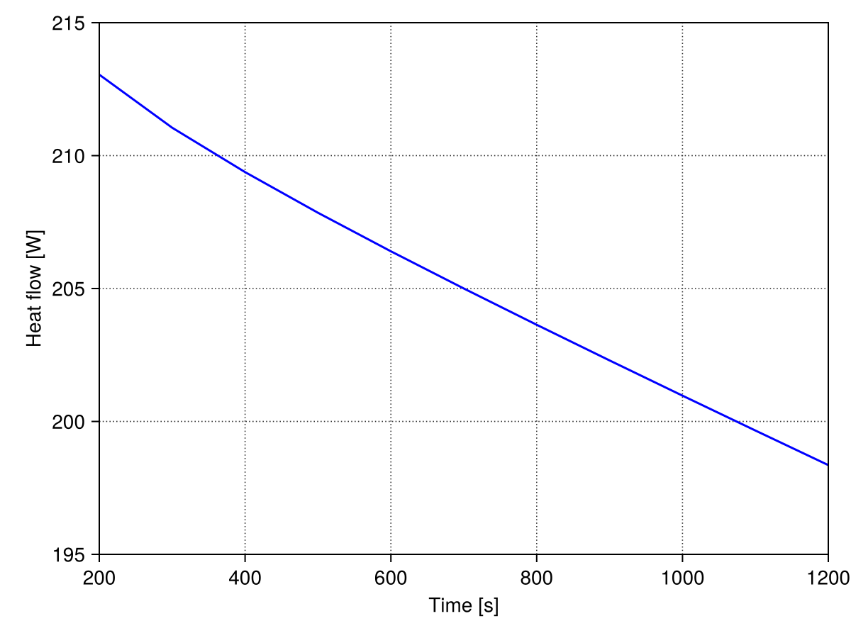
To get an integral value we used SaveScalars, which is plotted below against time. Since the value of heat flux was integrated over the boundary, it is provided in power units. At the final time we have a value of $Q\approx{}198.4\;W$. The segment of cylinder simulated here has an outer radius of $R=0.10\;m$ and height $h=0.05\;m$. With this values in hand it can be shown that the integral quantity is evaluated for $2\pi\;rad$, i.e. $Q=2\pi{}Rhq=Aq$.
For the 3D case most of the ideas still hold true. The main difference here is that no intrinsic symmetry was implied by the cartesian choice of formulation. Symmetries were enforced by boundary conditions. That means that computed quantities evaluate to the actual area of the wedge, here covering an angle of $\pi/4$ - what should be clear as it is common to most simulation packages.
Graphical post-processing
ParaView was employed to generate standard animations of temperature evolution in bodies. Below we have the 2D axisymmetric results:
The same was done for 3D equivalent case as illustrated next:
Classification
#elmer/domain/axisymmetric #elmer/domain/transient #elmer/models/heat-equation #elmer/models/save-line #elmer/models/save-scalars #elmer/models/result-output-solver #elmer/models/flux-solver