21 Fitting NASA9 data

The goal of this document is to provide a better understanding on how to fit empirical data to NASA9 parameterization of thermodynamic properties; more details are provided in the original NASA report. A progressive level of complexity is used to provide better insights of how the species thermodynamics is encoded in this format.

21.1 Helper utilities

21.2 Nitrogen actual fit

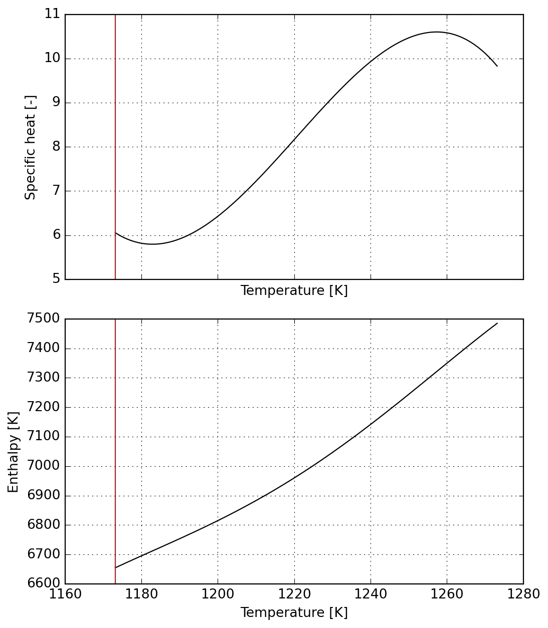
Below we display in text format an actual NASA9 fit taken from airNASA9.yaml data file provided with Cantera; this is a fully parameterized species, making it a bit more difficult to visually understand the role of different coefficients
The third coefficient \(a_{2}\) is related to the specific heat intercept when \(T=0\) and the eighth coefficient \(a_{7}\) represents the integration constant for providing enthalpy over a range
Since NASA9 functions are provided in dimensionless form, it is worth dividing computed values by ideal gas constant, so that values are in the same units as the provided coefficients

The next cell illustrates the dimensionless specific heat and enthalpy over a typical industrial range.

21.3 Enforcing constant specific heat

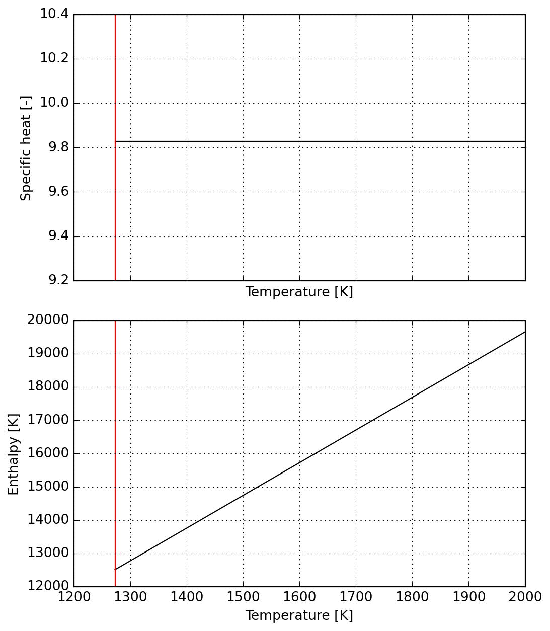
Next we create a dummy species (in Cantera composition needs to include actual atoms or you need to create a new database for elements) with all coefficients set to zero except those related to specific heat
This way we establish a piecewise-constant specific heat function; notice that doing so will produce thermodynamic inconsistent steps in enthalpy

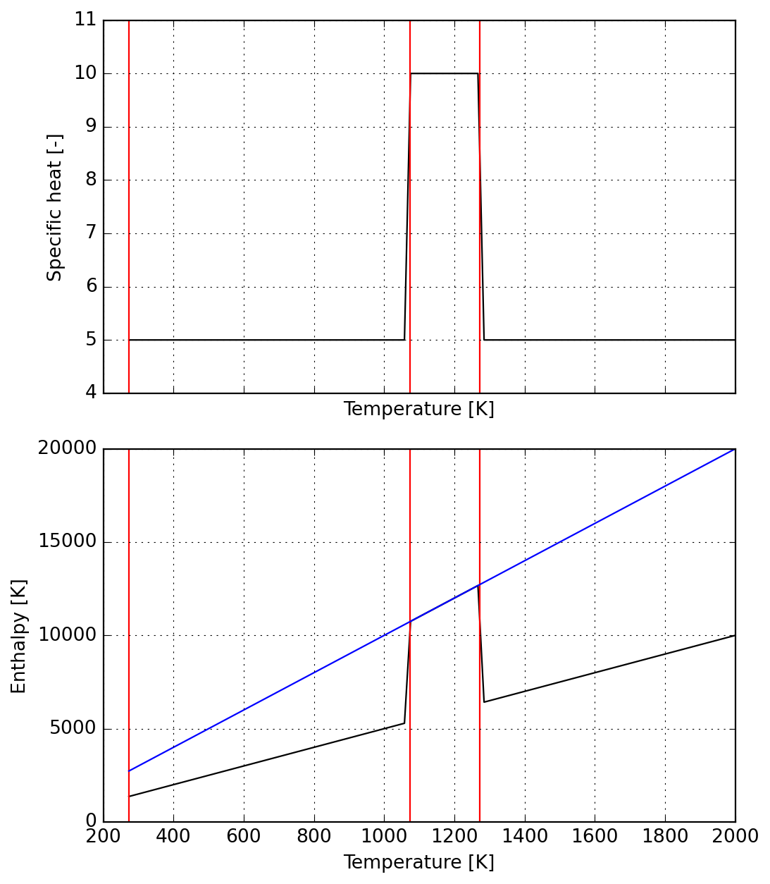
First, notice that the temperature ranges are closed-open ranges, meaning the first point belongs to the range but the last not; we introduce T_tol to compute a last value of enthalpy over each range as close as possible to the next
To ensure continuity of enthalpy function, we evaluate the gap h_hi-h_lo at each range end and add that to the correction of the previous range (as enthalpy is integrated from the reference temperature)
Using dh0 = s.dimless_h(298.15) to compute the initial value is optional and simply enforces zero enthalpy at the reference state, but in principle it won’t affect any computations as only enthalpy changes make sense physically

Note: as we are dealing with constant \(c_P\) here, we could have computed all the above enthalpy values straight from specific heat integration by hand, but this would be more complicated in general cases and it was chosen to present the more general (and with least user interaction) approach. See below that the enthalpy at reference temperature fits nicely with the specific heat provided above.

np.True_

Generalizing for all the steps, we could manually compute everything as follows:

((6856.5, np.float64(6856.500000000005)),
 (490.75, np.float64(490.75000000001455)))

21.4 Ensuring enthalpy continuity

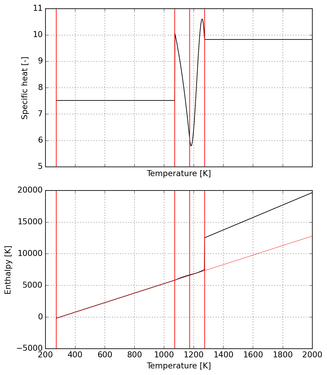
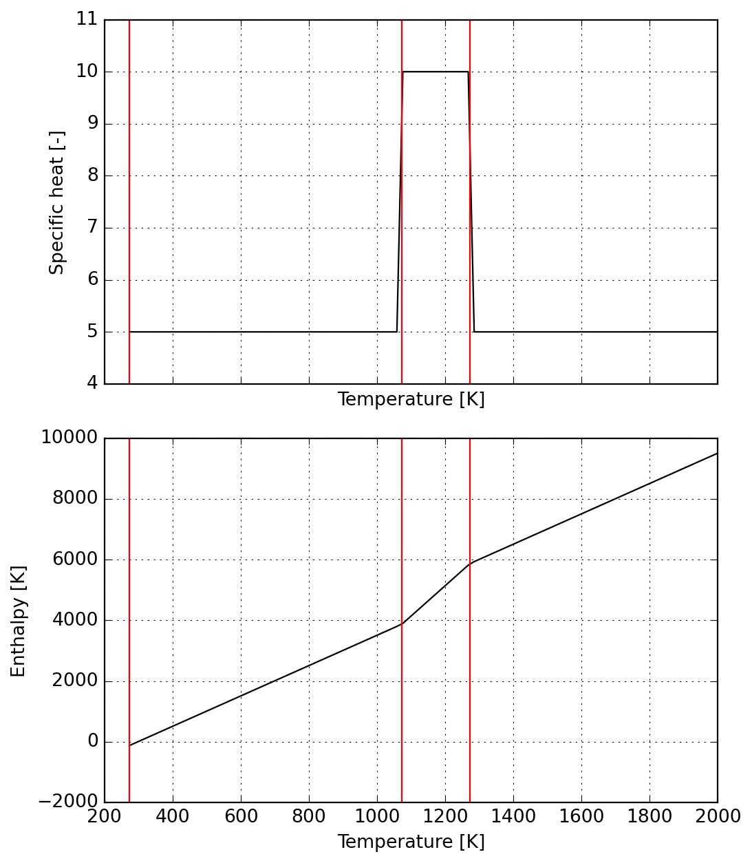
To wrap up, we use string interpolation to fix the integration constants required to ensure continuity of enthalpy function

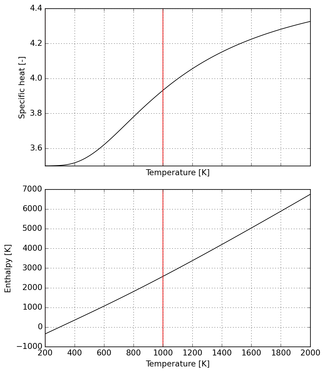
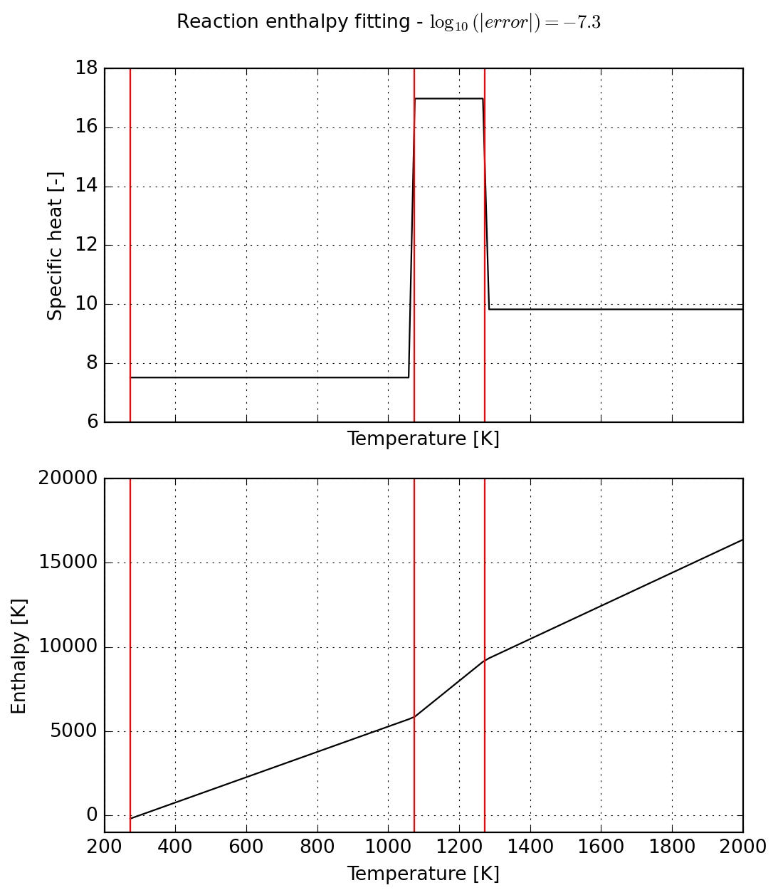
21.5 Application to a real material

We start by providing actual physical values to be converted into NASA9 format.

Calculations involve three phases (1) convert into units used by NASA9 format, (2) smearing of reaction enthalpy into specific heat, and (3) corrections required for continuity of enthalpy function.

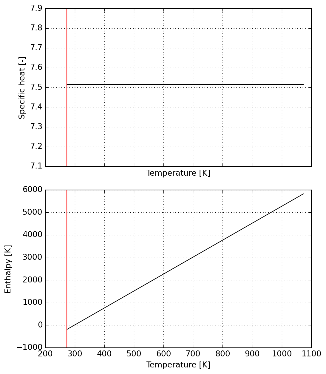
Alternative for using a constant specific heat over the whole range:

Next we generate the YAML input that will be used in Cantera database file.


name: meal
composition: {Si: 1, O: 2}
thermo:
  model: NASA9
  temperature-ranges: [273.15, 1073.15, 1273.15, 6000.0]
  data:
  - [ 0.00000000e+00,  0.00000000e+00,  7.51537686e+00,
      0.00000000e+00,  0.00000000e+00,  0.00000000e+00,
      0.00000000e+00, -2.24070961e+03,  0.00000000e+00]

  - [ 0.00000000e+00,  0.00000000e+00,  1.69746349e+01,
      0.00000000e+00,  0.00000000e+00,  0.00000000e+00,
      0.00000000e+00, -1.23919123e+04,  0.00000000e+00]

  - [ 0.00000000e+00,  0.00000000e+00,  9.82780051e+00,
      0.00000000e+00,  0.00000000e+00,  0.00000000e+00,
      0.00000000e+00, -3.29292018e+03,  0.00000000e+00]

name: meal
composition: {Si: 1, O: 2}
thermo:
  model: constant-cp
  cp0: 95.5200 J/mol/K
  h0: 0.0 J/mol®

Finally we inspect results before proceeding to use of newly fit data.

Important: NASA9 is the only parameterization supporting an arbitrary number of temperature ranges in Cantera. Given the number of parameters, it is expected to slow down simulations. For more details, please check the documentation.

21.6 Generalizing approach

Warning

Work in progress from here on… the code is right but the thermodynamics is pretty much sketchy!

We start by declaring the symbols for temperature t and model coefficients a:

The next cell provides the representations of specific heat capacity and enthalpy as described here. We also provide the derivatives of theses functions computed algorithmically with help of casadi.gradient.

Below we illustrate the symbolic computational graph of operations for checking the functions:

SX(((((a_0+(a_1*t))+(a_2*sq(t)))+(a_3*(t*sq(t))))+(a_4*sq(sq(t)))))

Below the reaction start we enforce a constant specific heat with zero enthalpy at reference temperature:

The reaction range is split in two parts, the first corresponding to a raising specific heat which reaches the maximum value.

DM([-1.81899e-12, -1.25056e-12])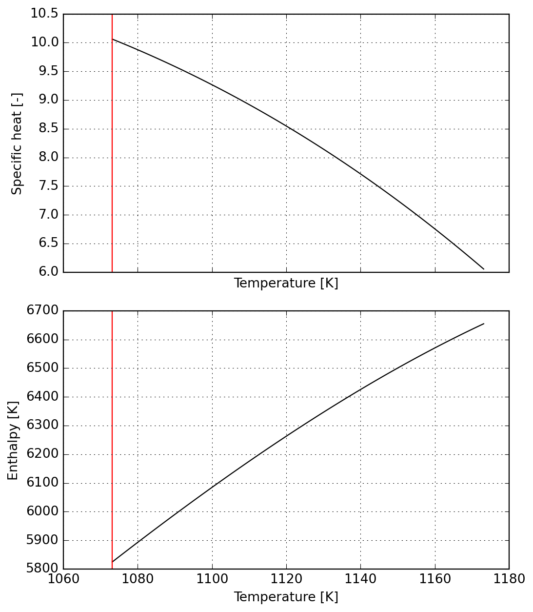

For the second part of the reaction we ensure continuity from the previous one

DM([-4.46699e-11, -1.13545e-11, 2.24354e-12, -1.10049e-09, -3.17539e-09])