2  Simulation

aka majordome.simulation

2.1 Elmer Multiphysics

2.1.1 TimeStepAccumulator

TimeStepAccumulator

TimeStepAccumulator(*time_steps : ConstantTimeStepInterval): -> None:

Helper for creating cumulative time steps in Elmer SIF files.

Parameters

*time_steps : ConstantTimeStepInterval

    Variable number of time step intervals to accumulate.

---

add_block

add_block(
    self : Any,
    *,
    duration : float | None = None,
    end_time : float | None = None,
    **kws : Any
    ) -> None:

Add a new block of time steps with the given parameters.

Parameters

duration : float | None = None

    Duration of the new time step block. If not provided, then end_time must be provided.

end_time : float | None = None

    End time of the new time step block. If not provided, then duration must be provided. If provided, the duration of the new block will be calculated as end_time - self.duration.

kws :  = None

    Additional keyword arguments to pass to the ConstantTimeStepInterval constructor.

---

append

append(
    self : Any,
    time_step : ConstantTimeStepInterval
    ) -> None:

Append a new time step to the accumulator.

Parameters

time_step : ConstantTimeStepInterval

    The time step interval to append to the accumulator.

---

to_dataframe

to_dataframe(self : Any): -> DataFrame:

Convert the accumulated time steps into a table.

---

In general the usage of the TimeStepAccumulator is as follows:

! >> Total duration: 0.001 << !
! Step Duration(3)     =         1e-05         9e-05        0.0009
Timestep Sizes(3)      =  1.000000e-06  1.000000e-05  1.000000e-04
Timestep Intervals(3)  =            10             9             9
Output Intervals(3)    =            10             9             9

2.1.1.1 ConstantTimeStepInterval

In some special cases, when using TimeStepAccumulator you might want to add time steps one by one, which can be done using the append method in combination with the ConstantTimeStepInterval described below.

ConstantTimeStepInterval

ConstantTimeStepInterval(
    duration : float,
    time_step : float | None = None,
    save_interval : float | None = None,
    *,
    min_steps : int = 2
    ) -> None:

Create a constant time step interval for a simulation.

Parameters

duration : float

    Total duration of the time step interval.

time_step : float | None = None

    Size of each time step. If not provided, it will be calculated based on the duration and min_steps parameters.

save_interval : float | None = None

    Interval at which to save results. If not provided, it will be set equal to time_step.

min_steps : int = 2

    Minimum number of time steps to use if time_step is not provided. Must be at least 1. Default is 2.

---

into_formatted_data

into_formatted_data(self : Any): -> list[str]:

Format the time step data for output in an Elmer SIF file.

---

2.1.2 ElmerConvergenceData

ElmerConvergenceData

ElmerConvergenceData(file_path : str | pathlib.Path): -> None:

Class for handling convergence data from Elmer simulations.

Parameters

file_path : str | pathlib.Path

    Path to the file containing convergence data, typically output by Elmer’s SaveLine solver.

---

get_solver_data

get_solver_data(
    self : Any,
    solver_id : int
    ) -> DataFrame:

Get convergence data for a specific solver.

Parameters

solver_id : int

    The ID of the solver to filter by.

---

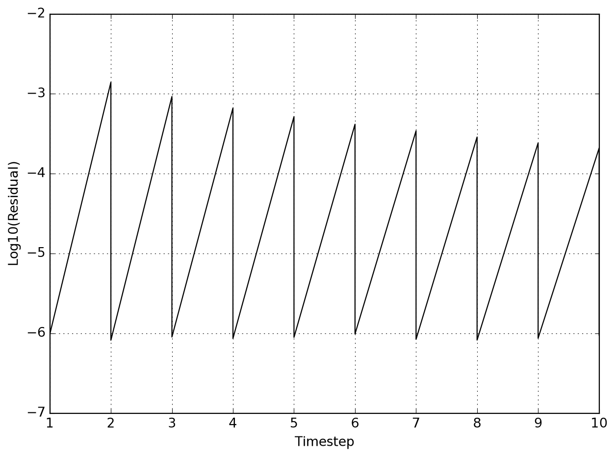
plot_solver_convergence

plot_solver_convergence(
    self : Any,
    *,
    solver_id : int,
    final_iter : bool = False,
    time_axis : NDArray | None = None,
    plot : majordome.utilities.plotting.MajordomePlot | None = None
    ) -> MajordomePlot:

Plot convergence data for a specific solver.

Parameters

solver_id : int

    The ID of the solver to plot.

final_iter : bool = False

    If True, only plot the final iteration for each timestep.

time_axis : NDArray | None = None

    Optional array of time values to use as the x-axis. If not provided, the timestep numbers will be used.

plot : majordome.utilities.plotting.MajordomePlot | None = None

    Placeholder for plot object provided by decorator.

---

tracked_solvers

tracked_solvers(self : Any): -> list[int]:

List of unique solvers tracked in the data.

---

2.1.3 ElmerTabularData

ElmerTabularData

ElmerTabularData(
    fname : str | pathlib.Path,
    *,
    fmeta : str | pathlib.Path | None = None
    ):

Class to represent the data of a SaveLine results file.

Parameters

fname : str | pathlib.Path

    The path to the data file output of Elmer’s SaveLine solver.

fmeta : str | pathlib.Path | None = None

    The path to the associated metadata file. If not provided, the class will attempt to find a metadata file in the same directory as the data file, with the same name but with a .names extension. If still not found, it will look for the metadata file one level above the data file directory.

---

metadata

metadata(self : Any): -> ElmerTabularMetadata:

Provides access to the metadata of the save line data.

---

data

data(self : Any): -> DataFrame:

Provides access to the data of the save line.

---

ElmerTabularMetadata

ElmerTabularMetadata(filepath : str | pathlib.Path)::

Class to hold metadata from Elmer SaveLine .names file.

Parameters

filepath : str | pathlib.Path

    Path to the .names metadata file.

---

metadata

metadata(self : Any): -> dict:

Return the metadata as a dictionary.

---

columns

columns(self : Any): -> dict:

Return the column definitions as a dictionary.

---

{'Metadata for SaveScalars file': 'results/tabular_np20.dat',
 'Elmer version': '26.1',
 'Elmer revision': 'Release',
 'Elmer compilation date': '2026-03-02',
 'Solver input file': 'case.sif',
 'File started at': '2026/03/18 16:03:05',
 'Variables in columns of matrix': '',
 'columns': {1: 'value: time scalar variable',
  2: 'nonlin converged: temperature',
  3: 'boundary sum: temperature loads over bc externalmask : mpi_sum',
  4: 'body mean: temperature mask bodymolten',
  5: 'body mean: temperature mask bodymould',
  6: 'body int: internal energy mask bodymolten : mpi_sum',
  7: 'body int: internal energy mask bodymould : mpi_sum',
  8: 'body volume: temperature mask bodymolten : mpi_sum',
  9: 'body int: density mask bodymolten : mpi_sum',
  10: 'body mean: density mask bodymolten'}}

	0	1	2	3	4
value: time scalar variable	1.000000e-02	2.000000e-02	3.000000e-02	4.000000e-02	5.000000e-02
nonlin converged: temperature	1.000000e+00	1.000000e+00	1.000000e+00	1.000000e+00	1.000000e+00
boundary sum: temperature loads over bc externalmask : mpi_sum	-3.109205e-11	2.515731e-12	8.600641e-12	4.978725e-11	1.465802e-11
body mean: temperature mask bodymolten	2.046525e+03	2.005741e+03	1.977803e+03	1.956194e+03	1.938414e+03
body mean: temperature mask bodymould	3.307690e+02	3.434748e+02	3.531031e+02	3.610606e+02	3.679436e+02
body int: internal energy mask bodymolten : mpi_sum	1.228442e+06	1.210679e+06	1.197206e+06	1.185981e+06	1.176250e+06
body int: internal energy mask bodymould : mpi_sum	1.198843e+04	2.743795e+04	3.957989e+04	4.990254e+04	5.903935e+04
body volume: temperature mask bodymolten : mpi_sum	1.300000e-04	1.300000e-04	1.300000e-04	1.300000e-04	1.300000e-04
body int: density mask bodymolten : mpi_sum	4.690027e-01	4.726299e-01	4.754619e-01	4.778310e-01	4.798897e-01
body mean: density mask bodymolten	3.828723e+03	3.883139e+03	3.919478e+03	3.947489e+03	3.970816e+03

2.2 Ansys Fluent

2.2.1 FluentFvParticlesParser

This class provides functionality for parsing particle track files. Fluent export DPM results in several formats; majordome supports fieldview particle tracks through FluentFvParticlesParser. Loading a file is as simple as:

You can retrieve the names of columns and number of individual tracks with the following properties:

(['x', 'y', 'z', 'residence_time', 'time_step'], 2)

For convenience, tracks can be recovered as data frames through object indexing:

	x	y	z	residence_time	time_step
0	0.128501	0.537214	-0.622358	0.000000	0.000000e+00
1	0.128493	0.537929	-0.619682	0.000107	1.697420e-07
2	0.128493	0.537964	-0.619554	0.000112	2.738057e-07
3	0.128488	0.538534	-0.617419	0.000176	4.008972e-07
4	0.128477	0.539842	-0.612481	0.000299	7.041471e-07

2.2.2 FluentInterpolationParser

Sometimes is is also useful to parse interpolation files. It enables one to compute new quantites for an interpolation files may be useful, especially in reasearch settings. Class FluentInterpolationParser is able to read the contents of an interpolation file exported in plain text format. Below you find an example of parsing.

             x0 in range (        11:        16)
             x1 in range (        17:        22)
       pressure in range (        23:        28)
     x-velocity in range (        29:        34)
     y-velocity in range (        35:        40)
    temperature in range (        41:        46)
              k in range (        47:        52)
          omega in range (        53:        58)

Names of variables are provided by property variable_names:

['x0',
 'x1',
 'pressure',
 'x-velocity',
 'y-velocity',
 'temperature',
 'k',
 'omega']

Valid names can be used to retrieve data for a given variable:

array([0.1, 0.1, 0.2, 0.3, 0.4])

The whole data table can be retreived with data property, where each variable correspond to a column:

array([[0.1, 1. , 9. , 9. , 9. , 9. , 9. , 9. ],
       [0.1, 2. , 1. , 1. , 1. , 1. , 1. , 1. ],
       [0.2, 3. , 2. , 2. , 2. , 2. , 2. , 2. ],
       [0.3, 4. , 3. , 3. , 3. , 3. , 3. , 3. ],
       [0.4, 5. , 4. , 4. , 4. , 4. , 4. , 4. ]])

2.3 Meshing

2.3.1 GmshOCCModel

GmshOCCModel

GmshOCCModel(
    *,
    render : bool = False,
    name : str = 'domain',
    config : dict[str, typing.Any] | None = None
    ) -> None:

Wrapper to manage OCC models with an OOP approach.

Parameters

render : bool = False

    Whether to launch the Gmsh GUI after building the model.

name : str = 'domain'

    Name of the Gmsh model.

config : dict[str, typing.Any] | None = None

    Provide configuration for gmsh internals.

---