from casadi import SX
from casadi import DM
from casadi import Function
from casadi import nlpsol
from casadi import vertcat
import numpy as np
import matplotlib.pyplot as plt13 Fundamentals of MPC
Let’s break down our introduction to model predictive control (MPC) into simpler blocks where we will study a parfect stirred reactor (PSR) model in transient mode.
13.1 A first MPC
In this study we implement a model predictive control (MPC) for a dummy chemical reactor. This notebook guides you through the different steps of the implementation using the powerful package CasADi in its Python programming interface.
Our goal is to provide controlled concentration output, which may be required to change in time, i.e. a costumer order required different concentratio, in a continuous stirred tank reactor.
In our dummy production, reagent \(A\) is fed to the system with a carrier \(B\) to produce \(C\), whose concentration is the target. The chemical process is illustrated as the irreversible reaction happening at a known rate \(k_1\):
\[ A + B \rightarrow B + C \]
To control the molar fraction of \(C\), denoted \(x_C\), we play with flow rates of \(A\) and \(B\) given by \(\dot{n}_A\) and \(\dot{n}_B\). For smooth functioning of the system, the total flow rate is required to remain constant at \(\dot{n}_t\) so that \(\dot{n}_B=\dot{n}_t-\dot{n}_A\), i.e. a compensation valve is the action we control. That implies we have a single degree of freedom in the actions we can take to pilot this simple system.
The reactor volume is kept constant at \(n_t\) moles. The following differential equation applies to each chemical species \(i\)
\[ n_t\dot{x}_i = \dot{n}_i - \dot{n}_t x_i + \dot{n}_{gen,i} \]
Here \(\dot{n}_{gen,B}\) is zero for \(B\) and is computed as a first order kinetic term \(\dot{n}_{gen,A}=-\dot{n}_{gen,C}=-k_1 x_A\) for other species.
Our tools:
To create the optimization routine we will make use of
SXsymbolic class ofcasadi.That will be used to compose right-hand side derivative
Functionobjects for later integrating the problem.Optimization of controls is done though solver Ipopt which can be accessed though interface
nlpsol.The reminder of imports are utilities that will be invoked at the right moment.
As stated in the introduction, some quantities are fixed/known. That includes the reaction rate \(k_1=10.0\:\mathrm{mol\cdotp{}s^{-1}}\), the size of reactor \(n_t=500.0\:\mathrm{mol}\) and the total flow rate of \(\dot{n}_t=3.0\:\mathrm{mol\cdotp{}s^{-1}}\). We declare them here so that we can focus on symbolic manipulations.
k_1 = 10.0
n_t = 500.0
ndot_t = 3.0
There are 3 chemical species being modeled in the fictional system.
Using SX we create their symbolic variables so that we can profit from casadi automatic differentiation.
This is helpful for computation of jacobian and hessian matrices required by the optimizer.
x_A = SX.sym("x_A")
x_B = SX.sym("x_B")
x_C = SX.sym("x_C")
The same is done for flow rate \(\dot{n}_A\) and restriction on total flow is applied.
Notice here that we can use numerical ndot_t and symbolic ndot_A in the same expression.
ndot_A = SX.sym("ndot_A")
ndot_B = ndot_t - ndot_A
Source terms are then computed as previously described.
Again we illustrate simultaneous use of symbolics and numerics.
rate = k_1 * x_A
ndot_gen_A = -rate
ndot_gen_B = 0.0
ndot_gen_C = +rate
With these elements we are ready to perform the molar balances describing the time-evolution of the system.
xdot_A = (ndot_A - ndot_t * x_A + ndot_gen_A) / n_t
xdot_B = (ndot_B - ndot_t * x_B + ndot_gen_B) / n_t
xdot_C = (0.0    - ndot_t * x_C + ndot_gen_C) / n_t
To create nice interfaces we group the variables in x and p.
It is common to use these names for the unknowns and control parameters is optimal control problem statements.
x = vertcat(x_A, x_B, x_C)
p = ndot_A
Using Function we wrap-up the above expressions.
Each function is provided a name, a list of inputs and a list of outputs.
Optional arguments are not used here to name the inputs and outputs and you can check their usage in the documentation.
F_xdot_A = Function("F_xdot_A", [x, p], [xdot_A])
F_xdot_B = Function("F_xdot_B", [x, p], [xdot_B])
F_xdot_C = Function("F_xdot_C", [x, p], [xdot_C])
It is interesting to check the string representation of a Function.
Here we see that it receives a first input i0 which is an array of 3 elements and a second number i1 for the returning a single value o0. As stated before, you can name these I/O using the more complete interface of Function.
F_xdot_AFunction(F_xdot_A:(i0[3],i1)->(o0) SXFunction)We can check the proper functioning of these functions as simple Python objects.
It shows that although we have symbolically built the system but numerical evaluation is possible.
Return values are of type DM, CasADi’s way of representing dense matrices (here an order zero matrix, a single number).
F_xdot_A([0.5, 0.5, 0], 10),\
F_xdot_B([0.5, 0.5, 0], 10),\
F_xdot_C([0.5, 0.5, 0], 10)
(DM(0.007), DM(-0.017), DM(0.01))The model being ready we can start the conception of our controller.
The numbers we need to choose here require domain-specific knowledge:
The first is the prediction horizon \(N_p\). It must be long enough so that the optimization routine foresees the dynamics of the system to apply corrections in time.
The horizon size alone has no sense without the definition of the time-step \(\tau\) between consective corrective actions. This again must take into consideration the delays system response and the valve itself in this specific case.
Here we chose to take into account the next 2000 s of the dynamics through 200 steps of 10 s.
You can check that given the aforementioned reactor size and flow rate, the characteristic time of the system is of the order of \(n_t/\dot{n}_t = 500\:\mathrm{mol} / 3\:\mathrm{mol\cdotp{}s^{-1}} \approx 170\:\mathrm{s}\), so the process window seems large enough to describe the full dilution of the system and the time step is less 10% of that time, what seems reasonable here.
Note: the time-step \(\tau\) may be the same used for integration of the problem, but you may use a smaller value if during each length \(\tau\) you keep the control action constant. This might be required when dealing with stiff differential equations of system model, i.e. a combustion process or complex gas pressure control.
Np = 200
tau = 10.0
The composition of the cost function in MPC also requires domain knowledge.
The scale of the problem is usually selected to be one of deviation of main controlled variable so the mutiplier of quadratic term \(Q\) is set to unity (or identity matrix in more complex multidimensional formulations).
We should also pay attention to the change in command, so another quadratic term penalizing important changes is added to cost function. Its scaling \(R\) has to be chosen so that is remains in a good order of magnitude compared to target variable cost and still perform its function.
The last parameter \(S\) is the terminal penalization, generally set to a high value so that we enforce the last point in prediction horizon to match the set-point.
Q = 1.0
R = 0.1
S = 100.0
Because of limitations of our compensation valve, the fraction of \(A\) in the total flow is limited to 90% of total feed rate.
Initially it is found to be at 50% of the total capacity and that will impact the first command change.
ndot_A_max = 0.9 * ndot_t
ndot_A_ini = 0.5 * ndot_t
Next we create our cost function J set initially to zero and the list of constraints g.
J = 0.0
g = []
The production planning already knows the target concentration (set-point) over the prediction horizon so that we can construct our cost function. It is symbolically declared in xs_C and contains one extra point over Np representing the current state of the reactor.
xs_C = SX.sym("xs_C", Np+1)We also need lower and upper boundaries, lbx and ubx, of our solution variable, here the controller command for the flow rate of \(A\). It can be set from zero up to the maximum amount it can be set, here 90% of total flow rate.
Note that constant numeric values could have been provided here, but for generality we will use a list here and feed it along with the integration so that you can see how one could implement a possibly varying control boundaries.
Same is done for the commands at each step sent to the valve.
lbx = []
ubx = []
v_ndot_A = []
The initial state of the system is set to the symbols we already know (later we will replace them by numeric measurements). Notice that in this tutorial case we are handling the variables individually, but in a real-world problem you would probably use a vector with all variables as we edd in x before.
xt_A, xt_B, xt_C = x_A, x_B, x_CFinally we integrate the problem over time. The loop is composed of a few characteristic steps:
Creation of a command variable
v_ndot_a_tsfor the current step.Bounding the values of control variable throughs
lbxandubx.Stacking of current system state in
xnand current commands inpn.Actual time integration of the system dynamics.
Increment of cost function with current deviations.
Add constraints (not done here) to the states and controls.
Below you will recognize a simple Euler time-stepping.
Again, in real-world problems you would at least use a Runge-Kutta order 4 integration. As it was said before, you might need to use an internal (smaller) time-step for very stiff problems, situation where the states
xnwould be internally updated but the commandpnwould be held constant.
In real-world you would probably use a multiple-shooting approach to simultaneously simulate and optimize the problem, if that is required. That comes with an additional computational cost because the optimization problem becomes larger. For keeping this tutorial focused on the main ideas it was chosen to exploit this simpler approach (from the implementation standpoint).
Since initial flow rate of \(A\) is already known and we are using R to avoid abrupt changes in the flow command, we make use of that value here to compute the initial step accordingly.
for ts in range(Np):
    v_ndot_A_ts = SX.sym(f"v_qdot_A_{ts}")
    v_ndot_A.append(v_ndot_A_ts)

    lbx.append(0.0)
    ubx.append(ndot_A_max)

    xn = vertcat(xt_A, xt_B, xt_C)
    pn = v_ndot_A_ts

    xt_A = xt_A + tau * F_xdot_A(xn, pn)
    xt_B = xt_B + tau * F_xdot_B(xn, pn)
    xt_C = xt_C + tau * F_xdot_C(xn, pn)

    v_prev = ndot_A_ini if ts == 0 else v_ndot_A[ts-1]

    # scale_error  = (xt_C - xs_C[ts]) / (xt_C + 1.0e-09)
    # scale_change = (v_prev - v_ndot_A_ts) / (v_prev + 1.0e-09)

    scale_error  = xt_C - xs_C[ts]
    scale_change = v_prev - v_ndot_A_ts

    cost_error = Q * pow(scale_error, 2)
    cost_change = R * pow(scale_change, 2)

    J += cost_error + cost_change
To complete the cost function, the terminal cost is added with scale S.
J += S * pow(xt_C - xs_C[-1], 2)The assembly of the system to be solved made below. Here we have chosen to optimize the problem with Ipopt as a nonlinear problem. In some cases you might wish to use a quadratic solver, but it imposes some limitations in problem formulation. You should do that when solving as a NLP is too slow for your problem. In CasADi’s representation f denotes the cost, x the free variables (the commands here), g the constraints list, and p the parameters, values that were left in symbolic form and we need to provide numerically. Here p is the array of set-points and the system initial state. Interface nlpsol allows for creating a solver, which may be used many times later.
nlp = {
    "f": J,
    "x": vertcat(*v_ndot_A),
    "g": vertcat(*g),
    "p": vertcat(xs_C, x)
}
solver = nlpsol("solver", "ipopt", nlp)
Below we see the interface of the solver with the sizes of the arrays we must provide.
solverFunction(solver:(x0[200],p[204],lbx[200],ubx[200],lbg[0],ubg[0],lam_x0[200],lam_g0[0])->(x[200],f,g[0],lam_x[200],lam_g[0],lam_p[204]) IpoptInterface)Let’s now compose the parameters array. For the set-point xs_C_num consider that you need the solution to be delivered with a concentration of 30% in the first 75 steps (3/4 of prediction horizon) of \(C\) and for the next lot the concetration must be increased to 60%. Below we create and array with that.
xs_C_num = np.zeros(Np+1)
xs_C_num[:3*Np//5] = 0.2
xs_C_num[3*Np//5:] = 0.5
At the initial time the system is composed only of \(B\), the second element in our composition array. With that we can merge the arrays in the format expected by the solver (as declared above) to provide p.
x0_num = [0.0, 1.0, 0.0]
p = [*xs_C_num, *x0_num]
Call of the solver is mostly trivial. If this is the first call to the solver, normally provide an initial guess composed of a fixed value that makes sense to your system. Here an array of ones was chosen. When using the solver in an actual control loop, generally the results of last call are provided. Since we have a single constraint in g, it suffices to provide lbg=ubg=0.0 to enforce the initial flow rate to the prescribed value. Call can be a bit verbose and you might want to log it in a production environment.
solution = solver(x0=np.ones(Np), p=p, lbx=lbx, ubx=ubx, lbg=0.0, ubg=0.0)
******************************************************************************
This program contains Ipopt, a library for large-scale nonlinear optimization.
 Ipopt is released as open source code under the Eclipse Public License (EPL).
         For more information visit https://github.com/coin-or/Ipopt
******************************************************************************

This is Ipopt version 3.14.11, running with linear solver MUMPS 5.4.1.

Number of nonzeros in equality constraint Jacobian...:        0
Number of nonzeros in inequality constraint Jacobian.:        0
Number of nonzeros in Lagrangian Hessian.............:    19902

Total number of variables............................:      200
                     variables with only lower bounds:        0
                variables with lower and upper bounds:      200
                     variables with only upper bounds:        0
Total number of equality constraints.................:        0
Total number of inequality constraints...............:        0
        inequality constraints with only lower bounds:        0
   inequality constraints with lower and upper bounds:        0
        inequality constraints with only upper bounds:        0

iter    objective    inf_pr   inf_du lg(mu)  ||d||  lg(rg) alpha_du alpha_pr  ls
   0  1.1258206e+01 0.00e+00 5.43e-01  -1.0 0.00e+00    -  0.00e+00 0.00e+00   0
   1  7.8092583e+00 0.00e+00 7.04e-02  -1.0 2.90e-01    -  8.32e-01 1.00e+00f  1
   2  2.8059021e+00 0.00e+00 2.75e-02  -1.7 6.10e-01    -  8.56e-01 1.00e+00f  1
   3  7.9735197e-01 0.00e+00 2.56e-02  -2.5 5.86e-01    -  8.30e-01 1.00e+00f  1
   4  4.6957248e-01 0.00e+00 3.89e-16  -2.5 3.47e-01    -  1.00e+00 1.00e+00f  1
   5  4.0610971e-01 0.00e+00 5.07e-04  -3.8 2.30e-01    -  9.51e-01 1.00e+00f  1
   6  3.9418705e-01 0.00e+00 4.22e-16  -3.8 1.36e-01    -  1.00e+00 1.00e+00f  1
   7  3.9075820e-01 0.00e+00 7.22e-05  -5.7 7.49e-02    -  9.74e-01 1.00e+00f  1
   8  3.9027053e-01 0.00e+00 3.03e-04  -5.7 2.86e-02    -  1.00e+00 8.39e-01f  1
   9  3.9017046e-01 0.00e+00 1.22e-06  -5.7 1.36e-02    -  1.00e+00 9.99e-01f  1
iter    objective    inf_pr   inf_du lg(mu)  ||d||  lg(rg) alpha_du alpha_pr  ls
  10  3.9015880e-01 0.00e+00 5.91e-05  -8.6 4.00e-03    -  1.00e+00 9.35e-01f  1
  11  3.9015679e-01 0.00e+00 1.11e-16  -8.6 1.96e-03    -  1.00e+00 1.00e+00f  1
  12  3.9015656e-01 0.00e+00 1.52e-16  -8.6 8.68e-04    -  1.00e+00 1.00e+00f  1
  13  3.9015654e-01 0.00e+00 1.47e-16  -8.6 3.48e-04    -  1.00e+00 1.00e+00f  1
  14  3.9015653e-01 0.00e+00 2.17e-16  -8.6 8.04e-05    -  1.00e+00 1.00e+00f  1

Number of Iterations....: 14

                                   (scaled)                 (unscaled)
Objective...............:   3.9015653462196176e-01    3.9015653462196176e-01
Dual infeasibility......:   2.1747432450719620e-16    2.1747432450719620e-16
Constraint violation....:   0.0000000000000000e+00    0.0000000000000000e+00
Variable bound violation:   0.0000000000000000e+00    0.0000000000000000e+00
Complementarity.........:   4.1114517841581608e-09    4.1114517841581608e-09
Overall NLP error.......:   4.1114517841581608e-09    4.1114517841581608e-09


Number of objective function evaluations             = 15
Number of objective gradient evaluations             = 15
Number of equality constraint evaluations            = 0
Number of inequality constraint evaluations          = 0
Number of equality constraint Jacobian evaluations   = 0
Number of inequality constraint Jacobian evaluations = 0
Number of Lagrangian Hessian evaluations             = 14
Total seconds in IPOPT                               = 0.062

EXIT: Optimal Solution Found.
      solver  :   t_proc      (avg)   t_wall      (avg)    n_eval
       nlp_f  |        0 (       0) 409.00us ( 27.27us)        15
  nlp_grad_f  |        0 (       0) 694.00us ( 43.37us)        16
  nlp_hess_l  |  37.00ms (  2.64ms)  41.20ms (  2.94ms)        14
       total  |  52.00ms ( 52.00ms)  62.11ms ( 62.11ms)         1
Below we recover the solution for reuse in system simulation. Observe that the simulation loop is essentially the same as the construction of the cost function but we implement just the time-stepping routines.
ndot_A_opt = solution["x"].full().ravel()

xt_A = np.zeros(Np+1)
xt_B = np.zeros(Np+1)
xt_C = np.zeros(Np+1)

xt_A[0] = x0_num[0]
xt_B[0] = x0_num[1]
xt_C[0] = x0_num[2]

for ts in range(1, Np+1):
    xn = vertcat(xt_A[ts-1], xt_B[ts-1], xt_C[ts-1])
    pn = ndot_A_opt[ts-1]

    xt_A[ts] = xt_A[ts-1] + tau * F_xdot_A(xn, pn)
    xt_B[ts] = xt_B[ts-1] + tau * F_xdot_B(xn, pn)
    xt_C[ts] = xt_C[ts-1] + tau * F_xdot_C(xn, pn)
According to the quality deparment, the product is good to be delivered if its concentration is anywhere withing 5% of the prescribed value. A boolean array good is created for displaying. This could be used to predict when the exit valve feed barrels of product or when it should recycle/throw the output.
xs_C_max = np.clip(xs_C_num + 0.05, 0.0, 1.0)
xs_C_min = np.clip(xs_C_num - 0.05, 0.0, 1.0)
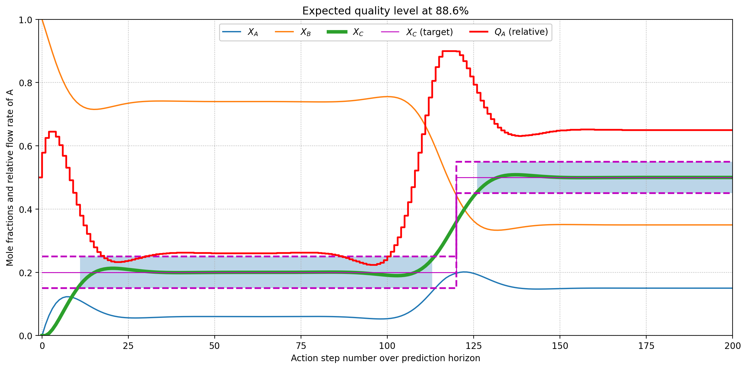
good = (xt_C >= xs_C_min) & (xt_C <= xs_C_max)The next figure illustrates the expected dynamical behavior of the system. First concentration of \(C\) rises from zero to the prescribed value in about 20 steps, and because of the change in set-point it starts deviating from target at step 60 to reach the new value. It is also interesting to observe that command saturates at 85%, what indicates that production of the second target is a limiting case for this reactor. We respected the process window during 58.4% of the time.
Because of how matplotlib.step works, to display properly the commands and responses we need to add an extra copy of last command to the end of the results. Using where="post" is also required so that a command starts at the reference time-step it is supposed to. You can check the plotting behaviour with the following snippet.
x = [1, 2, 3, 4]
y = [0, 1, 3, 1]

z = [1, 2, 0]
z.append(z[-1])

plt.plot(x, y, "o-", label="Response")
plt.step(x, z, "o-", label="Command", where="post")
plt.legend(loc=2)
steps = list(range(Np+1))
quality = 100 * sum(good.astype("u8")) / len(good)
cmd = list(ndot_A_opt / ndot_t)
cmd.append(cmd[-1])
plt.style.use("default")
plt.figure(figsize=(12, 6))
plt.grid(linestyle=":")
plt.plot(steps, xt_A, lw=2, label="$X_A$")
plt.plot(steps, xt_B, lw=2, label="$X_B$")
plt.plot(steps, xt_C, lw=4, label="$X_C$")
plt.step(steps, xs_C_max, "m--", lw=2, label="_none_", where="post")
plt.step(steps, xs_C_min, "m--", lw=2, label="_none_", where="post")
plt.step(steps, xs_C_num, "m-", lw=1, label="$X_C$ (target)", where="post")
# Add *negative time* with initial flow rate.
plt.step([-1, *steps], [ndot_A_ini/ ndot_t, *cmd], "r", lw=2,
label="$Q_A$ (relative)", where="post")
plt.fill_between(steps, xs_C_min, xs_C_max, where=good, alpha=0.3)
plt.title(f"Expected quality level at {quality:.1f}%")
plt.ylabel("Mole fractions and relative flow rate of A")
plt.xlabel("Action step number over prediction horizon")
plt.legend(loc="upper center", fancybox=True, framealpha=1.0, ncol=6)
plt.xlim(-1, Np)
plt.ylim(0, 1)
plt.tight_layout()
There are many ways you could propose exercises from this guided study:
- Implement a higher order time-stepping scheme.
- Provide simultaneous simulation/optimization with multiple-shooting.
- Investigate role of total flow rate or reactor size over quality.
- Increase error out of target value range (shadowed zones in figure).
- Use the solver in a simulated control loop with random noise in measurements.
- …
13.2 MPC code refactoring
13.2.1 Build system of equations
x = SX.sym("x", 3)
x
SX([x_0, x_1, x_2])ndot_tot = SX.sym("ndot_tot")
ndot = SX.sym("ndot", 3)
ndot[1] = ndot_tot - ndot[0]
ndot[2] = 0
ndotSX([ndot_0, (ndot_tot-ndot_0), 0])k = SX.sym("k")
rate = k * x[0]
rateSX((k*x_0))ndot_gen = vertcat(-rate, 0.0, rate)
ndot_genSX(@1=(k*x_0), [(-@1), 0, @1])n_tot = SX.sym("n_tot")
xdot = (ndot - ndot_tot * x + ndot_gen) / n_tot
xdotSX(@1=(k*x_0), [(((ndot_0-(ndot_tot*x_0))-@1)/n_tot), (((ndot_tot-ndot_0)-(ndot_tot*x_1))/n_tot), ((@1-(ndot_tot*x_2))/n_tot)])F_xdot = Function("F_xdot", [x, ndot[0], ndot_tot, n_tot, k], [xdot])F_xdotFunction(F_xdot:(i0[3],i1,i2,i3,i4)->(o0[3]) SXFunction)F_xdot([0.5, 0.5, 0.0], 10.0, 3.0, 1000.0, 10.0)DM([0.0035, -0.0085, 0.005])F_xdot(x, ndot[0], ndot_tot, n_tot, k * x[1])SX(@1=((k*x_1)*x_0), [(((ndot_0-(ndot_tot*x_0))-@1)/n_tot), (((ndot_tot-ndot_0)-(ndot_tot*x_1))/n_tot), ((@1-(ndot_tot*x_2))/n_tot)])13.2.2 Provide parameters
Np = 200
tau = 10.0

Q = 1.0
R = 0.1
S = 100.0

k_num = 10.0
n_tot_num = 500.0
ndot_tot_num = 3.0

ndot0_max = 0.9 * ndot_tot_num
ndot0_ini = 0.5 * ndot_tot_num

pars_fixed = [ndot_tot_num, n_tot_num, k_num]
13.2.3 Integrate symbolically
def step(xn, pn):
    return F_xdot(xn, pn, *pars_fixed)

def integrate(xn, pn):
    return xn + tau * step(xn, pn)
integrate(x, ndot0_ini)SX(@1=10, @2=1.5, @3=3, @4=(@1*x_0), @5=500, [(x_0+(@1*(((@2-(@3*x_0))-@4)/@5))), (x_1+(@1*((@2-(@3*x_1))/@5))), (x_2+(@1*((@4-(@3*x_2))/@5)))])J = 0.0
g = []
xs2 = SX.sym("xs2", Np+1)
lbx = []
ubx = []
v_ndot0 = []xn = x
for ts in range(Np):
v_ndot0_ts = SX.sym(f"v_ndot0_{ts}")
v_ndot0.append(v_ndot0_ts)
lbx.append(0.0)
ubx.append(ndot0_max)
xn = integrate(xn, v_ndot0_ts)
v_prev = ndot0_ini if ts == 0 else v_ndot0[ts-1]
scale_error = xn[2] - xs2[ts]
scale_change = v_prev - v_ndot0_ts
cost_error = Q * pow(scale_error, 2)
cost_change = R * pow(scale_change, 2)
J += cost_error + cost_change
J += S * pow(xn[2] - xs2[-1], 2)13.2.4 Optimize controls
nlp = {
    "f": J,
    "x": vertcat(*v_ndot0),
    "g": vertcat(*g),
    "p": vertcat(xs2, x)
}
solver = nlpsol("solver", "ipopt", nlp)solverFunction(solver:(x0[200],p[204],lbx[200],ubx[200],lbg[0],ubg[0],lam_x0[200],lam_g0[0])->(x[200],f,g[0],lam_x[200],lam_g[0],lam_p[204]) IpoptInterface)xs2_num = np.zeros(Np+1)
xs2_num[:3*Np//5] = 0.2
xs2_num[3*Np//5:] = 0.5x0_num = [0.0, 1.0, 0.0]
p = [*xs2_num, *x0_num]solution = solver(x0=np.ones(Np), p=p, lbx=lbx, ubx=ubx, lbg=0.0, ubg=0.0)This is Ipopt version 3.14.11, running with linear solver MUMPS 5.4.1.
Number of nonzeros in equality constraint Jacobian...: 0
Number of nonzeros in inequality constraint Jacobian.: 0
Number of nonzeros in Lagrangian Hessian.............: 19902
Total number of variables............................: 200
variables with only lower bounds: 0
variables with lower and upper bounds: 200
variables with only upper bounds: 0
Total number of equality constraints.................: 0
Total number of inequality constraints...............: 0
inequality constraints with only lower bounds: 0
inequality constraints with lower and upper bounds: 0
inequality constraints with only upper bounds: 0
iter objective inf_pr inf_du lg(mu) ||d|| lg(rg) alpha_du alpha_pr ls
0 1.1258206e+01 0.00e+00 5.43e-01 -1.0 0.00e+00 - 0.00e+00 0.00e+00 0
1 7.8092583e+00 0.00e+00 7.04e-02 -1.0 2.90e-01 - 8.32e-01 1.00e+00f 1
2 2.8059021e+00 0.00e+00 2.75e-02 -1.7 6.10e-01 - 8.56e-01 1.00e+00f 1
3 7.9735197e-01 0.00e+00 2.56e-02 -2.5 5.86e-01 - 8.30e-01 1.00e+00f 1
4 4.6957248e-01 0.00e+00 1.68e-16 -2.5 3.47e-01 - 1.00e+00 1.00e+00f 1
5 4.0610971e-01 0.00e+00 5.07e-04 -3.8 2.30e-01 - 9.51e-01 1.00e+00f 1
6 3.9418705e-01 0.00e+00 4.22e-16 -3.8 1.36e-01 - 1.00e+00 1.00e+00f 1
7 3.9075820e-01 0.00e+00 7.22e-05 -5.7 7.49e-02 - 9.74e-01 1.00e+00f 1
8 3.9027053e-01 0.00e+00 3.03e-04 -5.7 2.86e-02 - 1.00e+00 8.39e-01f 1
9 3.9017046e-01 0.00e+00 1.22e-06 -5.7 1.36e-02 - 1.00e+00 9.99e-01f 1
iter objective inf_pr inf_du lg(mu) ||d|| lg(rg) alpha_du alpha_pr ls
10 3.9015880e-01 0.00e+00 5.91e-05 -8.6 4.00e-03 - 1.00e+00 9.35e-01f 1
11 3.9015679e-01 0.00e+00 1.19e-16 -8.6 1.96e-03 - 1.00e+00 1.00e+00f 1
12 3.9015656e-01 0.00e+00 2.06e-16 -8.6 8.68e-04 - 1.00e+00 1.00e+00f 1
13 3.9015654e-01 0.00e+00 1.47e-16 -8.6 3.48e-04 - 1.00e+00 1.00e+00f 1
14 3.9015653e-01 0.00e+00 1.66e-16 -8.6 8.04e-05 - 1.00e+00 1.00e+00f 1
Number of Iterations....: 14
(scaled) (unscaled)
Objective...............: 3.9015653462196181e-01 3.9015653462196181e-01
Dual infeasibility......: 1.6593394627301955e-16 1.6593394627301955e-16
Constraint violation....: 0.0000000000000000e+00 0.0000000000000000e+00
Variable bound violation: 0.0000000000000000e+00 0.0000000000000000e+00
Complementarity.........: 4.1114517841593586e-09 4.1114517841593586e-09
Overall NLP error.......: 4.1114517841593586e-09 4.1114517841593586e-09
Number of objective function evaluations = 15
Number of objective gradient evaluations = 15
Number of equality constraint evaluations = 0
Number of inequality constraint evaluations = 0
Number of equality constraint Jacobian evaluations = 0
Number of inequality constraint Jacobian evaluations = 0
Number of Lagrangian Hessian evaluations = 14
Total seconds in IPOPT = 0.060
EXIT: Optimal Solution Found.
solver : t_proc (avg) t_wall (avg) n_eval
nlp_f | 1.00ms ( 66.67us) 395.00us ( 26.33us) 15
nlp_grad_f | 0 ( 0) 678.00us ( 42.37us) 16
nlp_hess_l | 28.00ms ( 2.00ms) 40.14ms ( 2.87ms) 14
total | 63.00ms ( 63.00ms) 60.60ms ( 60.60ms) 113.2.5 Post-processing
ndot0_opt = solution["x"].full().ravel()

xt = np.zeros((Np+1, 3))
xt[0, :] = x0_num

xn = xt[0]

for ts in range(1, Np+1):
    xn = integrate(xn, ndot0_opt[ts-1])
    xt[ts] = xn.full().ravel()
xs2_max = np.clip(xs2_num + 0.05, 0.0, 1.0)
xs2_min = np.clip(xs2_num - 0.05, 0.0, 1.0)
good = (xt[:, 2] >= xs2_min) & (xt[:, 2] <= xs2_max)
steps = list(range(Np+1))
quality = 100 * sum(good.astype("u8")) / len(good)
cmd = list(ndot0_opt / ndot_tot_num)
cmd.append(cmd[-1])
plt.style.use("default")
fig = plt.figure(figsize=(12, 6))
plt.grid(linestyle=":")
plt.plot(steps, xt[:, 0], label="$X_A$")
plt.plot(steps, xt[:, 1], label="$X_B$")
plt.plot(steps, xt[:, 2], lw=4, label="$X_C$")
plt.step(steps, xs2_max, "m--", lw=2, label="_none_", where="post")
plt.step(steps, xs2_min, "m--", lw=2, label="_none_", where="post")
plt.step(steps, xs2_num, "m-", lw=1, label="$X_C$ (target)", where="post")
# Add *negative time* with initial flow rate.
plt.step([-1, *steps], [ndot0_ini/ ndot_tot_num, *cmd], "r", lw=2,
label="$Q_A$ (relative)", where="post")
plt.fill_between(steps, xs2_min, xs2_max, where=good, alpha=0.3)
plt.title(f"Expected quality level at {quality:.1f}%")
plt.ylabel("Mole fractions and relative flow rate of A")
plt.xlabel("Action step number over prediction horizon")
plt.legend(loc="upper center", fancybox=True, framealpha=1.0, ncol=6)
plt.xlim(-1, Np)
plt.ylim(0, 1)
plt.tight_layout()
13.3 Wrapping up MPC
13.3.1 Create models
class PlantModel:
    """ Minimal implementation of system dynamics. """
    def __init__(self):
        x = SX.sym("x", 3) # Concentrations
        k = SX.sym("k", 1) # Rate constant
        N = SX.sym("N", 1) # System size

        # Total flow rate.
        Ndot = SX.sym("Ndot", 1)

        # Feed flow rates.
        ndot = SX.sym("ndot", 3)
        ndot[1] = Ndot - ndot[0]
        ndot[2] = 0

        # Production rates of species.
        vdot = k * x[0] * DM([-1, 0, 1])

        # Symbolic balance equation.
        xdot = (ndot - Ndot * x + vdot) / N

        # Functional balance equation.
        xrhs = Function(
            "xdot",
            [x, ndot[0], Ndot, N, k],
            [xdot],
            ["x", "ndot_A", "Ndot", "N", "k"],
            ["xdot"]
        )

        self._states = x
        self._balance_eqns_sym = xdot
        self._balance_eqns_fun = xrhs

    @property
    def states(self):
        return self._states

    @property
    def balance_eqns_sym(self):
        return self._balance_eqns_sym

    @property
    def balance_eqns_fun(self):
        return self._balance_eqns_fun
class InstantiatedPlant:
""" Instantiation of dynamics with fixed parameters. """
def __init__(self, model, k, N, Ndot, tau):
self._states = model.states
self._rhs = model.balance_eqns_fun
self._pars = [Ndot, N, k]
self._tau = tau
@property
def states(self):
return self._states
def step_euler(self, xn, pn):
return xn + self._tau * self._rhs(xn, pn, *self._pars)class ControlsMPC:
""" A simple MPC for a given plant. """
def __init__(self, plant, Np, R, S):
self._plant = plant
self._horizon = Np
# TODO instead of computing cost directly in _integrate
# just store the values in arrays and provide these
# in optimize so that we can play for parametrization.
self._R = R
self._S = S
self._p = SX.sym("p", Np+1)
self._xp = SX.sym("xp", Np+1)
self._x0 = SX.sym("x0", 3, 1)
self._xt = SX.sym("xt", 3, Np+1)
self._xt[:, 0] = self._x0
J, F = self._integrate()
self._cost = J
self._sim = F
def _integrate(self):
print("Initial call to MPC: symbolic integration")
J = 0
x = self._xt[:, 0]
for ts in range(1, self._horizon+1):
x = self._plant.step_euler(x, self._p[ts])
self._xt[:, ts] = x
# TODO: implement an actual scaling so that both have
# the same magnitude and Q, R become scale-independent!
scale_error = x[2] - self._xp[ts]
scale_change = self._p[ts] - self._p[ts-1]
# scale_error /= (x[2] + 1.0e-15)
# scale_change /= (self._p[ts] + 1.0e-15)
cost_error = pow(scale_error, 2)
cost_change = self._R * pow(scale_change, 2)
J += cost_error + cost_change
J += self._S * pow(x[2] - self._xp[-1], 2)
F = Function("sim", [self._x0, self._p], [self._xt])
return J, F
def optimize(self, x0, p0, xsp, pmax):
# Constraint *negative time* command to the current value.
g = [self._p[0] - p0]
# XXX: abuse of notation! Notice below that the dictionary
# *unknowns* "x" are set to `self._p`, while *parameters*
# "p" are given the *x's*. This is because we are finding
# the optimal controls here and already know the target
# profile and initial states for concentrations *x*!
solver = nlpsol("solver", "ipopt", {
"f": self._cost,
"x": self._p,
"g": vertcat(*g),
"p": vertcat(self._xp, self._x0)
})
p = [*xsp, *x0]
guess = np.ones(self._horizon+1)
solution = solver(x0=guess, p=p, lbx=0, ubx=pmax, lbg=0, ubg=0)
popt = solution["x"].full().ravel()
xt = self._sim(x0, popt).full().T
return popt, xt, solution13.3.2 Solution workflow
- Create dynamics
model = PlantModel()
model.balance_eqns_fun
Function(xdot:(x[3],ndot_A,Ndot,N,k)->(xdot[3]) SXFunction)- Provide parameters
k = 10.0
N = 500.0
Ndot = 3.0

ndot_A_max = 0.9 * Ndot
ndot_A_ini = 0.5 * Ndot

Np = 200
tau = 10.0

R = 0.1
S = 100.0

x0 = [0.0, 1.0, 0.0]

xsp = np.zeros(Np+1)
xsp[:3*Np//5] = 0.2
xsp[3*Np//5:] = 0.5- Setup controller
plant = InstantiatedPlant(model, k, N, Ndot, tau)

mpc = ControlsMPC(plant, Np, R, S)
Initial call to MPC: symbolic integration- Optimize and retrieve results
popt, xt, solution = mpc.optimize(x0, ndot_A_ini, xsp, ndot_A_max)This is Ipopt version 3.14.11, running with linear solver MUMPS 5.4.1.
Number of nonzeros in equality constraint Jacobian...: 1
Number of nonzeros in inequality constraint Jacobian.: 0
Number of nonzeros in Lagrangian Hessian.............: 19904
Total number of variables............................: 201
variables with only lower bounds: 0
variables with lower and upper bounds: 201
variables with only upper bounds: 0
Total number of equality constraints.................: 1
Total number of inequality constraints...............: 0
inequality constraints with only lower bounds: 0
inequality constraints with lower and upper bounds: 0
inequality constraints with only upper bounds: 0
iter objective inf_pr inf_du lg(mu) ||d|| lg(rg) alpha_du alpha_pr ls
0 1.1289480e+01 5.00e-01 5.43e-01 -1.0 0.00e+00 - 0.00e+00 0.00e+00 0
1 7.8535959e+00 0.00e+00 2.21e-01 -1.0 5.00e-01 - 7.07e-01 1.00e+00f 1
2 3.6890341e+00 0.00e+00 1.19e-01 -1.7 4.83e-01 - 7.75e-01 1.00e+00f 1
3 1.2029735e+00 0.00e+00 3.97e-02 -2.5 4.59e-01 - 7.70e-01 1.00e+00f 1
4 5.4417451e-01 0.00e+00 6.69e-03 -2.5 4.00e-01 - 9.27e-01 1.00e+00f 1
5 4.1843093e-01 0.00e+00 1.16e-03 -3.8 2.60e-01 - 9.31e-01 1.00e+00f 1
6 3.9726342e-01 0.00e+00 5.56e-16 -3.8 1.69e-01 - 1.00e+00 1.00e+00f 1
7 3.9147600e-01 0.00e+00 1.46e-04 -5.7 1.02e-01 - 9.58e-01 1.00e+00f 1
8 3.9034658e-01 0.00e+00 1.77e-04 -5.7 4.13e-02 - 1.00e+00 9.11e-01f 1
9 3.9018244e-01 0.00e+00 5.13e-05 -5.7 1.78e-02 - 1.00e+00 9.72e-01f 1
iter objective inf_pr inf_du lg(mu) ||d|| lg(rg) alpha_du alpha_pr ls
10 3.9016625e-01 0.00e+00 2.24e-16 -5.7 5.31e-03 - 1.00e+00 1.00e+00f 1
11 3.9015738e-01 0.00e+00 3.42e-05 -8.6 2.57e-03 - 1.00e+00 9.43e-01f 1
12 3.9015662e-01 0.00e+00 1.33e-16 -8.6 1.28e-03 - 1.00e+00 1.00e+00f 1
13 3.9015655e-01 0.00e+00 1.50e-16 -8.6 5.36e-04 - 1.00e+00 1.00e+00f 1
14 3.9015655e-01 0.00e+00 1.86e-16 -8.6 1.69e-04 - 1.00e+00 1.00e+00f 1
Number of Iterations....: 14
(scaled) (unscaled)
Objective...............: 3.9015654580404924e-01 3.9015654580404924e-01
Dual infeasibility......: 1.8607716730850261e-16 1.8607716730850261e-16
Constraint violation....: 0.0000000000000000e+00 0.0000000000000000e+00
Variable bound violation: 0.0000000000000000e+00 0.0000000000000000e+00
Complementarity.........: 9.6345181304803798e-09 9.6345181304803798e-09
Overall NLP error.......: 9.6345181304803798e-09 9.6345181304803798e-09
Number of objective function evaluations = 15
Number of objective gradient evaluations = 15
Number of equality constraint evaluations = 15
Number of inequality constraint evaluations = 0
Number of equality constraint Jacobian evaluations = 15
Number of inequality constraint Jacobian evaluations = 0
Number of Lagrangian Hessian evaluations = 14
Total seconds in IPOPT = 0.059
EXIT: Optimal Solution Found.
solver : t_proc (avg) t_wall (avg) n_eval
nlp_f | 0 ( 0) 372.00us ( 24.80us) 15
nlp_g | 0 ( 0) 17.00us ( 1.13us) 15
nlp_grad_f | 0 ( 0) 616.00us ( 38.50us) 16
nlp_hess_l | 31.00ms ( 2.21ms) 40.34ms ( 2.88ms) 14
nlp_jac_g | 0 ( 0) 8.00us (500.00ns) 16
total | 63.00ms ( 63.00ms) 59.06ms ( 59.06ms) 1- Display results
xsp_max = np.clip(xsp + 0.05, 0.0, 1.0)
xsp_min = np.clip(xsp - 0.05, 0.0, 1.0)
good = (xt[:, 2] >= xsp_min) & (xt[:, 2] <= xsp_max)

steps = list(range(Np+1))
quality = 100 * sum(good.astype("u8")) / len(good)

cmd = list(popt / Ndot)
cmd.append(cmd[-1])

plt.style.use("default")
fig = plt.figure(figsize=(12, 6))
plt.grid(linestyle=":")

plt.plot(steps, xt[:, 0], label="$X_A$")
plt.plot(steps, xt[:, 1], label="$X_B$")
plt.plot(steps, xt[:, 2], lw=4, label="$X_C$")

plt.step(steps, xsp_max, "m--", lw=2, label="_none_", where="post")
plt.step(steps, xsp_min, "m--", lw=2, label="_none_", where="post")
plt.step(steps, xsp, "m-", lw=1, label="$X_C$ (target)", where="post")
plt.fill_between(steps, xsp_min, xsp_max, where=good, alpha=0.3)

plt.step([-1, *steps], cmd, "r", lw=2, label="$Q_A$ (relative)", where="post")

plt.title(f"Expected quality level at {quality:.1f}%")
plt.ylabel("Mole fractions and relative flow rate of A")
plt.xlabel("Action step number over prediction horizon")
plt.legend(loc="upper center", fancybox=True, framealpha=1.0, ncol=6)
plt.xlim(-1, Np)
plt.ylim(0, 1)
plt.tight_layout()