%load_ext autoreload
%autoreload 27 Fitting NASA9 data
The goal of this document is to provide a better understanding on how to fit empirical data to NASA9 parameterization of thermodynamic properties; more details are provided in the original NASA report. A progressive level of complexity is used to provide better insights of how the species thermodynamics is encoded in this format.
from textwrap import dedent, indent
from casadi import SX, DM, Function
from casadi import vertcat, dot, log, gradient, nlpsol
from majordome import Capturing, MajordomePlot, bounds
import cantera as ct
import numpy as np
C:\Users\walte\GitHub\majordome\notes\.venv\Lib\site-packages\rsciio\utils\rgb_tools.py:46: VisibleDeprecationWarning: The module `rsciio.utils.rgb_tools` has been renamed to `rsciio.utils.rgb` and it will be removed in version 1.0.
warnings.warn(
C:\Users\walte\GitHub\majordome\notes\.venv\Lib\site-packages\rsciio\utils\tools.py:93: VisibleDeprecationWarning: ensure_directory has been moved to `rsciio.utils.path` and will be removed from `rsciio.utils.tools` in version 1.0.
warnings.warn(message, VisibleDeprecationWarning)
C:\Users\walte\GitHub\majordome\notes\.venv\Lib\site-packages\rsciio\utils\tools.py:93: VisibleDeprecationWarning: append2pathname has been moved to `rsciio.utils.path` and will be removed from `rsciio.utils.tools` in version 1.0.
warnings.warn(message, VisibleDeprecationWarning)
C:\Users\walte\GitHub\majordome\notes\.venv\Lib\site-packages\rsciio\utils\tools.py:93: VisibleDeprecationWarning: incremental_filename has been moved to `rsciio.utils.path` and will be removed from `rsciio.utils.tools` in version 1.0.
warnings.warn(message, VisibleDeprecationWarning)
C:\Users\walte\GitHub\majordome\notes\.venv\Lib\site-packages\tqdm\auto.py:21: TqdmWarning: IProgress not found. Please update jupyter and ipywidgets. See https://ipywidgets.readthedocs.io/en/stable/user_install.html
from .autonotebook import tqdm as notebook_tqdm
C:\Users\walte\GitHub\majordome\notes\.venv\Lib\site-packages\rsciio\utils\tools.py:93: VisibleDeprecationWarning: ensure_directory has been moved to `rsciio.utils.path` and will be removed from `rsciio.utils.tools` in version 1.0.
warnings.warn(message, VisibleDeprecationWarning)
C:\Users\walte\GitHub\majordome\notes\.venv\Lib\site-packages\rsciio\utils\tools.py:93: VisibleDeprecationWarning: overwrite has been moved to `rsciio.utils.path` and will be removed from `rsciio.utils.tools` in version 1.0.
warnings.warn(message, VisibleDeprecationWarning)7.1 Helper utilities
class Species:
    """ Helper species representation with graphical support. """
    __slots__ = ("species", "_c", "_h")

    def __init__(self, yaml_str: str) -> None:
        self.species = ct.Species.from_yaml(yaml_str)
        self._c = np.vectorize(self.species.thermo.cp)
        self._h = np.vectorize(self.species.thermo.h)

    def dimless_cp(self, T):
        """ Dimensionless specific heat. """
        return self._c(T) / ct.gas_constant

    def dimless_h(self, T):
        """ Dimensionless enthalpy. """
        return self._h(T) / ct.gas_constant

    @property
    def jumps(self):
        """ Provides access to temperature jumps. """
        return self.species.thermo.input_data["temperature-ranges"]

    @MajordomePlot.new(shape=(2, 1), size=(7, 8))
    def plot(self, *, T_lims, n_points=100, plot=None):
        """ Helper function to plot specific heat/enthalpy. """
        T = np.linspace(*T_lims, n_points)
        c = self.dimless_cp(T)
        h = self.dimless_h(T)

        fig, ax = plot.subplots()

        ax[0].plot(T, c, color="k")
        ax[1].plot(T, h, color="k")

        ax[0].set_xlabel("Temperature [K]")
        ax[1].set_xlabel("Temperature [K]")

        ax[0].set_ylabel("Specific heat [-]")
        ax[1].set_ylabel("Enthalpy [K]")

        for v in filter(lambda v: v < T[-1], self.jumps):
            ax[0].axvline(v, color="r")
            ax[1].axvline(v, color="r")
def formatted_nasa9_range(a):
""" Provide data for a single temperature interval. """
if len(a) == 6:
a = [0, 0, *a]
if len(a) != 8:
raise RuntimeError("There must be 8 coefficients!")
entry = dedent(f"""\
- [{a[0]:>15.8e}, {a[1]:>15.8e}, {a[2]:>15.8e},
{a[3]:>15.8e}, {a[4]:>15.8e}, {a[5]:>15.8e},
{a[6]:>15.8e}, {a[7]:>15.8e}, 0.00000000e+00]
""")
return entry
def formatted_yaml_for_test(As, Ts):
""" Formatted YAML species coefficients. """
data = dedent(f"""
name: meal
composition: {{Si: 1, O: 2}}
thermo:
model: NASA9
temperature-ranges: {Ts}
data:
""")
for a in As:
data += indent(formatted_nasa9_range(a), " ")
data += "\n"
return data7.2 Nitrogen actual fit
Below we display in text format an actual NASA9 fit taken from
airNASA9.yamldata file provided with Cantera; this is a fully parameterized species, making it a bit more difficult to visually understand the role of different coefficientsThe third coefficient \(a_{2}\) is related to the specific heat intercept when \(T=0\) and the eighth coefficient \(a_{7}\) represents the integration constant for providing enthalpy over a range
Since NASA9 functions are provided in dimensionless form, it is worth dividing computed values by ideal gas constant, so that values are in the same units as the provided coefficients
data = """
name: N2
composition: {N: 2}
thermo:
  model: NASA9
  temperature-ranges: [200.0, 1000.0, 6000.0, 2.0e+04]
  data:
  - [ 2.210371497e+04, -3.818461820e+02,  6.082738360e+00,
     -8.530914410e-03,  1.384646189e-05, -9.625793620e-09,
      2.519705809e-12,  7.108460860e+02, -1.076003744e+01]

  - [ 5.877124060e+05, -2.239249073e+03,  6.066949220e+00,
     -6.139685500e-04,  1.491806679e-07, -1.923105485e-11,
      1.061954386e-15,  1.283210415e+04, -1.586640027e+01]

  - [ 8.310139160e+08, -6.420733540e+05,  2.020264635e+00,
     -3.065092046e-02,  2.486903333e-06, -9.705954110e-11,
      1.437538881e-15,  4.938707040e+06, -1.672099740e+03]

note: Ref-Elm. Gurvich,1978 pt1 p280 pt2 p207. [tpis78]
"""
The next cell illustrates the dimensionless specific heat and enthalpy over a typical industrial range.
s = Species(data)
plot = s.plot(T_lims=(200, 2000))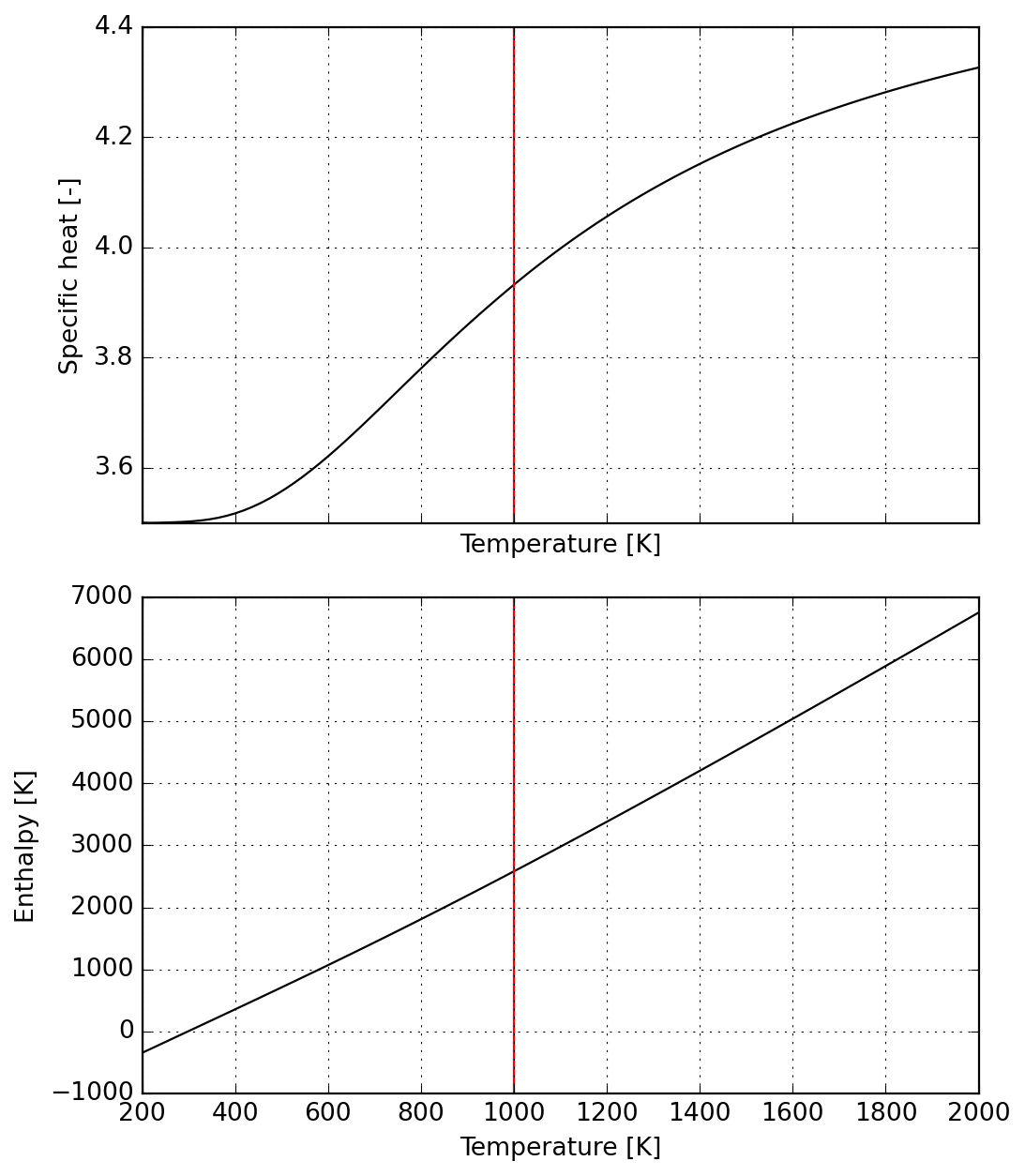
7.3 Enforcing constant specific heat
Next we create a dummy species (in Cantera composition needs to include actual atoms or you need to create a new database for elements) with all coefficients set to zero except those related to specific heat
This way we establish a piecewise-constant specific heat function; notice that doing so will produce thermodynamic inconsistent steps in enthalpy
data = """
name: dummy
composition: {N: 2}
thermo:
  model: NASA9
  temperature-ranges: [273.15, 1073.15, 1273.15, 6000.0]
  data:
  - [ 0.00000000e+00,  0.00000000e+00,  5.00000000e+00,
      0.00000000e+00,  0.00000000e+00,  0.00000000e+00,
      0.00000000e+00,  0.00000000e+00,  0.00000000e+00]

  - [ 0.00000000e+00,  0.00000000e+00,  1.00000000e+01,
      0.00000000e+00,  0.00000000e+00,  0.00000000e+00,
      0.00000000e+00,  0.00000000e+00,  0.00000000e+00]

  - [ 0.00000000e+00,  0.00000000e+00,  5.00000000e+00,
      0.00000000e+00,  0.00000000e+00,  0.00000000e+00,
      0.00000000e+00,  0.00000000e+00,  0.00000000e+00]
"""
s = Species(data)
plot = s.plot(T_lims=(s.jumps[0], 2000))
_ = plot.axes[0].set_ylim(4, 11)
T = np.linspace(s.jumps[0], 2000, 100)
_ = plot.axes[1].plot(T, 10 * T)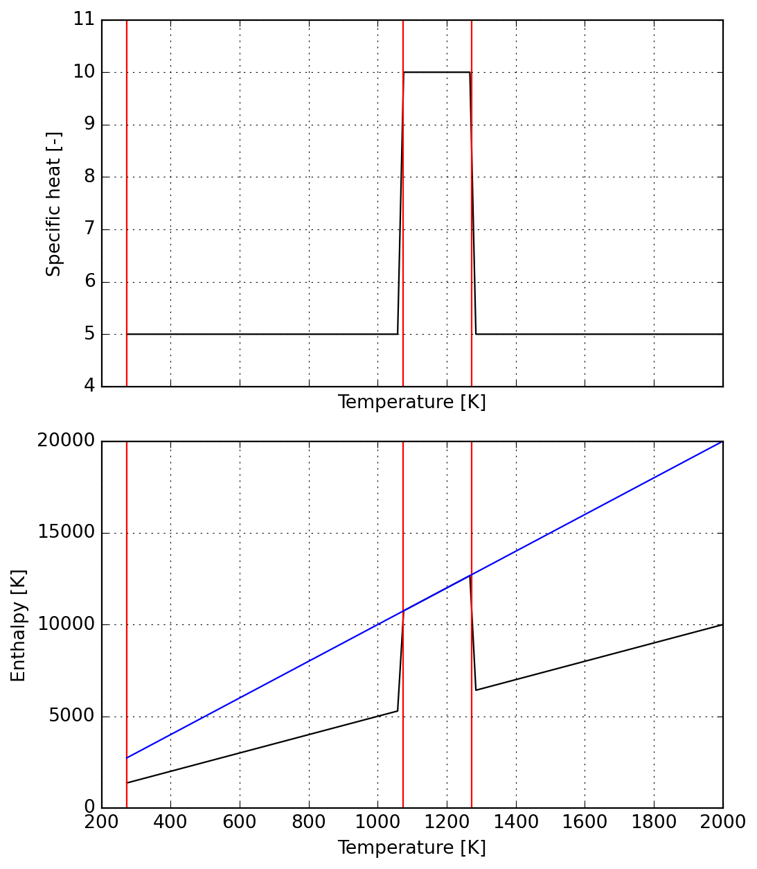
First, notice that the temperature ranges are closed-open ranges, meaning the first point belongs to the range but the last not; we introduce
T_tolto compute a last value of enthalpy over each range as close as possible to the nextTo ensure continuity of enthalpy function, we evaluate the gap
h_hi-h_loat each range end and add that to the correction of the previous range (as enthalpy is integrated from the reference temperature)Using
dh0 = s.dimless_h(298.15)to compute the initial value is optional and simply enforces zero enthalpy at the reference state, but in principle it won’t affect any computations as only enthalpy changes make sense physically
T_tol = 1.0e-12
T_ref = 298.15

h_hi = list(map(s.dimless_h, s.jumps))
h_lo = list(map(lambda t: s.dimless_h(t-T_tol), s.jumps))

dh0 = s.dimless_h(T_ref)
dh1 = dh0 + h_hi[1] - h_lo[1]
dh2 = dh1 + h_hi[2] - h_lo[2]
Note: as we are dealing with constant \(c_P\) here, we could have computed all the above enthalpy values straight from specific heat integration by hand, but this would be more complicated in general cases and it was chosen to present the more general (and with least user interaction) approach. See below that the enthalpy at reference temperature fits nicely with the specific heat provided above.
np.isclose(1.0, dh0 / (s.dimless_cp(T_ref) * T_ref))np.True_Generalizing for all the steps, we could manually compute everything as follows:
cp_0 = 5
cp_1 = 10
cp_2 = 5

h0 = cp_0 * T_ref
h1 = h0 + (cp_1 - cp_0) * s.jumps[1]
h2 = h1 + (cp_2 - cp_1) * s.jumps[2]

(h1, dh1), (h2, dh2)
((6856.5, np.float64(6856.500000000005)),
(490.75, np.float64(490.75000000001455)))7.4 Ensuring enthalpy continuity
- To wrap up, we use string interpolation to fix the integration constants required to ensure continuity of enthalpy function
data = f"""
name: N2
composition: {{N: 2}}
thermo:
  model: NASA9
  temperature-ranges: [273.15, 1073.15, 1273.15, 6000.0]
  data:
  - [ 0.00000000e+00,  0.00000000e+00,  5.00000000e+00,
      0.00000000e+00,  0.00000000e+00,  0.00000000e+00,
      0.00000000e+00,  {-dh0:.8e},  0.00000000e+00]

  - [ 0.00000000e+00,  0.00000000e+00,  1.00000000e+01,
      0.00000000e+00,  0.00000000e+00,  0.00000000e+00,
      0.00000000e+00,  {-dh1:.8e},  0.00000000e+00]

  - [ 0.00000000e+00,  0.00000000e+00,  5.00000000e+00,
      0.00000000e+00,  0.00000000e+00,  0.00000000e+00,
      0.00000000e+00,  {-dh2:.8e},  0.00000000e+00]
"""
s = Species(data)
plot = s.plot(T_lims=(s.jumps[0], 2000))
_ = plot.axes[0].set_ylim(4, 11)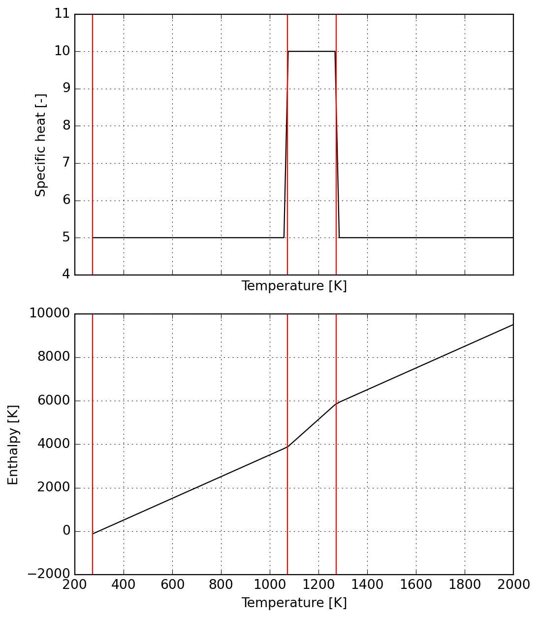
7.5 Application to a real material
We start by providing actual physical values to be converted into NASA9 format.
# Reference molecular mass [kg/kmol]
# XXX: arbitrary (but mandatory) for Cantera to convert units only!
mw_base = 60.083

# Material baseline specific heat [J/(kg.K)]
cp_base0 = 1040.0
cp_base2 = 1360.0

# Reaction enthalpy [J/kg]
dh_base = 229_800

# Reaction interval [K]
Tc_1 = 1073.15
Tc_2 = 1273.15
Calculations involve three phases (1) convert into units used by NASA9 format, (2) smearing of reaction enthalpy into specific heat, and (3) corrections required for continuity of enthalpy function.
# Reaction mid-point [K]
Tc_m = (Tc_1 + Tc_2) / 2

# [J/kg] * [kg/kmol] / [J/(kmol.K)] -> [K]
dh = dh_base * mw_base / ct.gas_constant

# For the following cp calculations we have:
# [J/(kg.K)] * [kg/kmol] / [J/(kmol.K)] -> [1]

# Range (0): baseline specific heat:
cp_0 = cp_base0 * mw_base / ct.gas_constant

# Range (2): baseline specific heat:
cp_2 = cp_base2 * mw_base / ct.gas_constant

# Range (1): baseline + smeared enthalpy:
cp_1p = 0.5 * (cp_0 + cp_2)
cp_1  = cp_1p + dh / (Tc_2 - Tc_1)

# Enforce enthalpy continuity:
dh0 = cp_0 * T_ref
dh1 = dh0 + (cp_1 - cp_0) * Tc_1
dh2 = dh1 + (cp_2 - cp_1) * Tc_2
Alternative for using a constant specific heat over the whole range:
cp_alt = cp_base2 + dh_base / (1000 - 0)
cp_alt *= mw_base / 1000
Next we generate the YAML input that will be used in Cantera database file.
data = f"""
name: meal
composition: {{Si: 1, O: 2}}
thermo:
  model: NASA9
  temperature-ranges: [273.15, {Tc_1}, {Tc_2}, 6000.0]
  data:
  - [ 0.00000000e+00,  0.00000000e+00,  {cp_0:.8e},
      0.00000000e+00,  0.00000000e+00,  0.00000000e+00,
      0.00000000e+00, {-dh0: .8e},  0.00000000e+00]

  - [ 0.00000000e+00,  0.00000000e+00,  {cp_1:.8e},
      0.00000000e+00,  0.00000000e+00,  0.00000000e+00,
      0.00000000e+00, {-dh1: .8e},  0.00000000e+00]

  - [ 0.00000000e+00,  0.00000000e+00,  {cp_2:.8e},
      0.00000000e+00,  0.00000000e+00,  0.00000000e+00,
      0.00000000e+00, {-dh2: .8e},  0.00000000e+00]
"""
print(data)
name: meal
composition: {Si: 1, O: 2}
thermo:
  model: NASA9
  temperature-ranges: [273.15, 1073.15, 1273.15, 6000.0]
  data:
  - [ 0.00000000e+00,  0.00000000e+00,  7.51537686e+00,
      0.00000000e+00,  0.00000000e+00,  0.00000000e+00,
      0.00000000e+00, -2.24070961e+03,  0.00000000e+00]

  - [ 0.00000000e+00,  0.00000000e+00,  1.69746349e+01,
      0.00000000e+00,  0.00000000e+00,  0.00000000e+00,
      0.00000000e+00, -1.23919123e+04,  0.00000000e+00]

  - [ 0.00000000e+00,  0.00000000e+00,  9.82780051e+00,
      0.00000000e+00,  0.00000000e+00,  0.00000000e+00,
      0.00000000e+00, -3.29292018e+03,  0.00000000e+00]
data_alt = f"""\
name: meal
composition: {{Si: 1, O: 2}}
thermo:
  model: constant-cp
  cp0: {cp_alt:.4f} J/mol/K
  h0: 0.0 J/mol®
"""
print(data_alt)
name: meal
composition: {Si: 1, O: 2}
thermo:
model: constant-cp
cp0: 95.5200 J/mol/K
h0: 0.0 J/mol®
Finally we inspect results before proceeding to use of newly fit data.
s = Species(data)
dh_glob = s.dimless_h(Tc_2) - s.dimless_h(Tc_1)
dh_sens = cp_1p * (Tc_2 - Tc_1)
dh_reac = dh_glob - dh_sens
dh_calc = ct.gas_constant * dh_reac / mw_base
error = np.log10(abs((dh_calc - dh_base) / dh_base))
title = f"Reaction enthalpy fitting - $\\log_{{10}}(|error|)={error:.1f}$ "
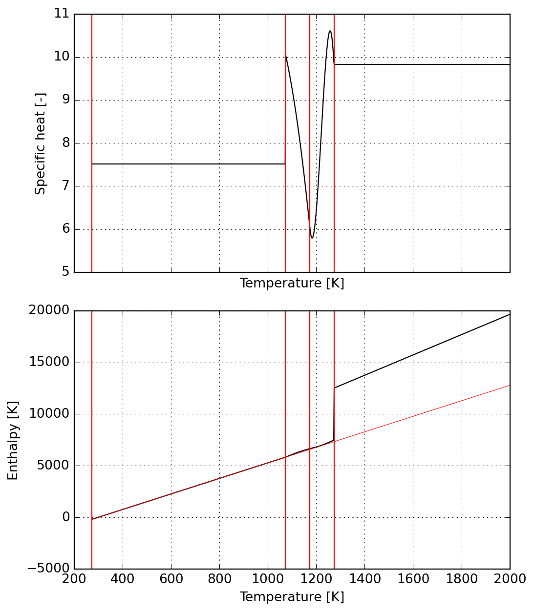
plot = s.plot(T_lims=(s.jumps[0], 2000))
_ = plot.axes[0].set_ylim(6, 18)
_ = plot.axes[1].set_ylim(-1000, 20000)
_ = plot.figure.suptitle(title)
_ = plot.figure.tight_layout()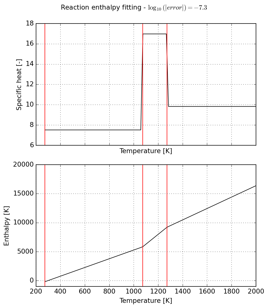
Important: NASA9 is the only parameterization supporting an arbitrary number of temperature ranges in Cantera. Given the number of parameters, it is expected to slow down simulations. For more details, please check the documentation.
7.6 Generalizing approach
Warning
Work in progress from here on… the code is right but the thermodynamics is pretty much sketchy!
We start by declaring the symbols for temperature t and model coefficients a:
t = SX.sym("t")
a = SX.sym("a", 6)
The next cell provides the representations of specific heat capacity and enthalpy as described here. We also provide the derivatives of theses functions computed algorithmically with help of casadi.gradient.
# Guess for parameters fitting (all zeros):
x0 = DM.zeros(a.numel())

match a.numel():
    case 8:
        # Full problem specification as per NASA9 format:
        coef_c = a[:-1]
        coef_h = vertcat(-a[0], a[1], a[2], a[3]/2, a[4]/3, a[5]/4, a[6]/5, a[7])
        temp_c = vertcat(t**(-2), t**(-1), 1, t, t**2, t**3, t**4)
        temp_h = vertcat(t**(-2), t**(-1) * log(t), 1, t, t**2, t**3, t**4, t**(-1))

    case 6:
        # Removing first two terms 1/T**n (set to zero in YAML data!):
        coef_c = a[:-1]
        coef_h = vertcat(a[0], a[1]/2, a[2]/3, a[3]/4, a[4]/5, a[5])
        temp_c = vertcat(1, t, t**2, t**3, t**4)
        temp_h = vertcat(1, t, t**2, t**3, t**4, t**(-1))

    case _:
        raise RuntimeError("Please, handle your modified polynomial above!")

# Inner products to compose c/R and h/RT
c_R  = dot(coef_c, temp_c)
h_RT = dot(coef_h, temp_h)

# NASA9 functions:
fn_c = Function("c", [t, a], [c_R])
fn_h = Function("h", [t, a], [t * h_RT])

# Derivative of specific heat for slope continuity:
fn_cdot = Function("cdot", [t, a], [gradient(c_R, t)])
fn_hdot = Function("hdot", [t, a], [gradient(t * h_RT, t)])
Below we illustrate the symbolic computational graph of operations for checking the functions:
display(fn_c(t, a))
# display(fn_h(t, a))
# display(fn_cdot(t, a))
# display(fn_hdot(t, a))SX(((((a_0+(a_1*t))+(a_2*sq(t)))+(a_3*(t*sq(t))))+(a_4*sq(sq(t)))))Below the reaction start we enforce a constant specific heat with zero enthalpy at reference temperature:
a1 = np.zeros(a.numel())
a1[0] = cp_0
a1[5] -= 298.15 * cp_0

T_lims = (273.15, Tc_1)
data = formatted_yaml_for_test([a1], list(T_lims))

s1 = Species(data)
plot = s1.plot(T_lims=T_lims)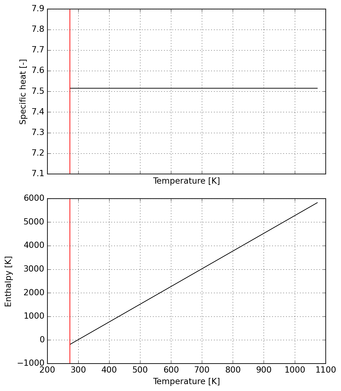
The reaction range is split in two parts, the first corresponding to a raising specific heat which reaches the maximum value.
nlp = {
    "x": a,
    "f": 1,
    "g": vertcat(
        # Null derivatives
        # fn_cdot(Tc_1, a),
        # fn_cdot(Tc_m, a),

        # Fixed specific heat/enthalpy
        # fn_c(Tc_1, a) - cp_0,

        fn_h(Tc_1, a) - s1.dimless_h(Tc_1),
        (fn_h(Tc_m, a) - fn_h(Tc_1, a)) - dh/2,
        # fn_h(Tc_m, a) - (s1.dimless_h(Tc_1) + dh/2),
    )
}

with Capturing() as out:
    solver = nlpsol("solver", "ipopt", nlp)
    sol = solver(x0=x0, lbg=0, ubg=0)

# Check if constraint violation remain acceptable:
display(sol["g"])

a2 = sol["x"].full().ravel()

T_lims = (Tc_1, Tc_m)
data = formatted_yaml_for_test([a2], list(T_lims))

s2 = Species(data)
plot = s2.plot(T_lims=T_lims)
DM([1.81899e-12, -3.41061e-13])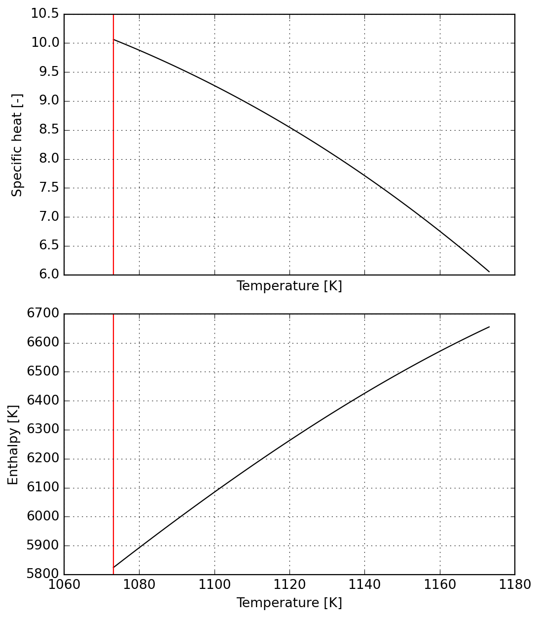
For the second part of the reaction we ensure continuity from the previous one
nlp = {
    "x": a,
    "f": 1,
    "g": vertcat(
        # Null derivatives
        fn_cdot(Tc_m, a) - fn_cdot(Tc_m, a2),
        # fn_cdot(Tc_2, a),

        # Fixed specific heat/enthalpy
        fn_c(Tc_m, a) - s2.dimless_cp(Tc_m),
        fn_c(Tc_2, a) - cp_2,

        fn_h(Tc_m, a) - s2.dimless_h(Tc_m),
        (fn_h(Tc_2, a) - fn_h(Tc_m, a)) - dh/2,
        # fn_h(Tc_2, a) - (s2.dimless_h(Tc_m) + dh/2),
    )
}

with Capturing() as out:
    solver = nlpsol("solver", "ipopt", nlp)
    sol = solver(x0=x0, lbg=0, ubg=0)

# Check if constraint violation remain acceptable:
display(sol["g"])

a3 = sol["x"].full().ravel()

T_lims = (Tc_m, Tc_2)
data = formatted_yaml_for_test([a3], list(T_lims))

s3 = Species(data)
plot = s3.plot(T_lims=T_lims)
DM([-6.74596e-09, -5.60689e-10, -2.45139e-10, 2.10093e-09, -1.1654e-09])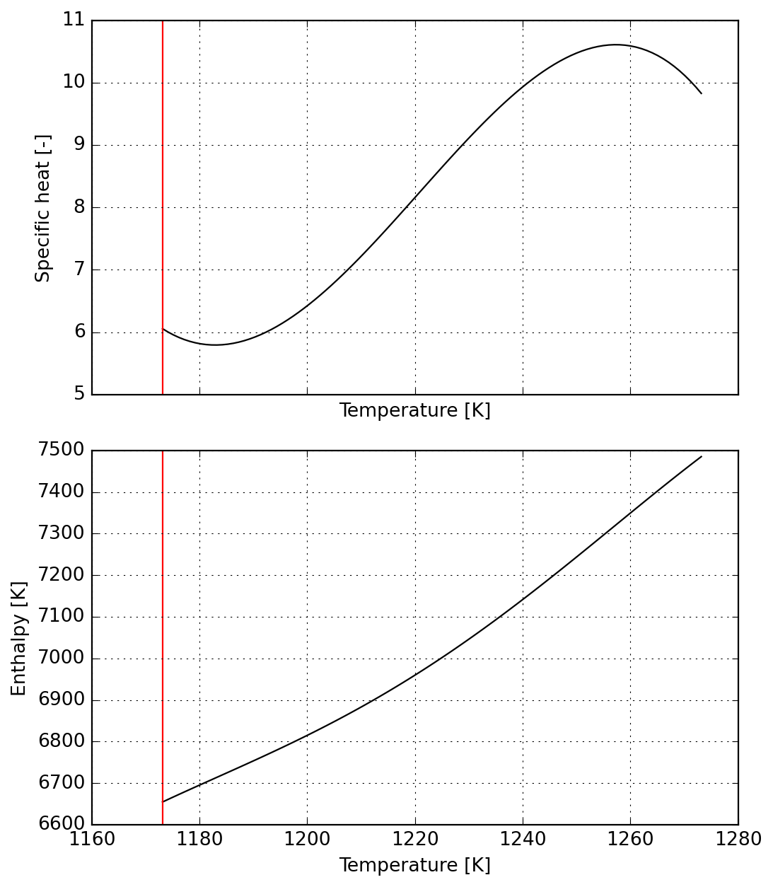
a4 = np.zeros(a.numel())
a4[0] = cp_2
# a4[5] -= (s3.dimless_h(Tc_2))# - s1.dimless_h(T_ref))

T_lims = (Tc_2, 2000.0)
data = formatted_yaml_for_test([a4], list(T_lims))

s4 = Species(data)
plot = s4.plot(T_lims=T_lims)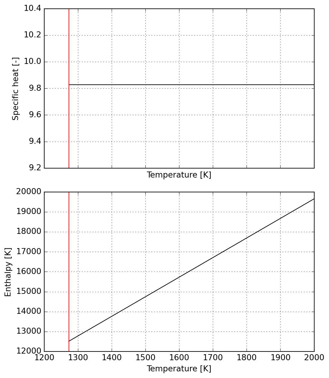
T_ch = [273.15, Tc_1, Tc_m, Tc_2, 2000.0]
data = formatted_yaml_for_test([a1, a2, a3, a4], T_ch)

s = Species(data)
plot = s.plot(T_lims=bounds(T_ch), n_points=1000)

T = np.linspace(*bounds(T_ch), 100)
_ = plot.axes[1].plot(T, cp_0 * (T - T_ref), c="r", lw=0.5)
# _ = plot.axes[1].set_xlim(1000, 1300)