30 Julia 101
Welcome to Julia 101! Julia from zero to hero (for Scientific Computing)!
Important: the following course may assume you are using a redistributable version of Julia packaged as described here. This might be useful for instructors willing to work without internet access.
In this first course you will be introduced to the Julia programming languange. By the end of the working session (~4h) you will be able to:
- understand what is Julia and its context of usage for Scientific Computing
- the difference between an interpreted and a compiled programming language
- use Julia as a calculator and program some simple functions
- read tabular data, perform some basic operations, and plot results
- learn the path towards searching information and package documentation
Our goal in this course is not to master Julia or even pretend you have learned it; we will open the gates so that you can go out there and solve problems by yourself (or maybe open Pandora’s box…).
This is probably your first time learning Julia. If you got here by other means than the main index, please consider reading the introduction of this document. Next, you can launch a terminal and try running Julia by simply typing julia and pressing return. For this introductory course I assume you are using VS Code for which you might also wish to install the recommended extensions.
30.1 REPL basics
Julia’s REPL (read-eval-print loop) is an interactive environment where you execute code as you write. It’s main goal is to manage Julia, test code snippets, get help, and launch larger chunks of code.
To enter the package manager mode press ]m to get help for a function or module press ?. Shell mode (system dependent) is accessed through ;, but you are discouraged to do so here. To get back to Julia interpreted simply press backspace.
- Below we inspect the status of our environment from the package manager:
(101) pkg> status
Status `D:\julia101\src\101\Project.toml`
  [13f3f980] CairoMakie v0.12.16
  [a93c6f00] DataFrames v1.7.0
  [c3e4b0f8] Pluto v0.20.3
[6099a3de] PythonCall v0.9.23- In help mode you can check how to use the
methodsfunction:
help?> methods
search: methods Method methodswith hasmethod

  methods(f, [types], [module])

  Return the method table for f.

  If types is specified, return an array of methods whose types match. If module is specified, return an
  array of methods defined in that module. A list of modules can also be specified as an array.

  │ Julia 1.4
  │
  │  At least Julia 1.4 is required for specifying a module.

  See also: which, @which and methodswith.
Try by yourself and run add Polynomials from package manager mode (we will need it later); what do you get if you check the status again?
30.2 Julia as a calculator
The following example should speak by itself:
julia> 1 + 1
2

julia> 2 * 3
6

julia> 3 / 4
0.75

julia> 3 // 4
3//4

julia> 3^3
27
The representation of numbers in the computer is not perfect and round-off may be a problem in some cases. The most common numeric types in Julia are illustrated below with help of typeof.
julia> typeof(1)
Int64

julia> typeof(1.0)
Float64

julia> typeof(3/4)
Float64

julia> typeof(3//4)
Rational{Int64}
Being a language conceived for numerical purposes, Julia has built-in support to complex numbers:
julia> 1 + 1im
1 + 1im

julia> typeof(1 + 1im)
Complex{Int64}
Some transcendental constants are also available:
julia> pi
π = 3.1415926535897...

julia> π
π = 3.1415926535897...

julia> typeof(pi)
Irrational{:π}

julia> Base.MathConstants.

catalan     e           eulergamma
eval        golden      include
pi          γ           π
φ           ℯ

julia> Base.MathConstants.e
ℯ = 2.7182818284590...

julia> names(MathConstants)
10-element Vector{Symbol}:
 :MathConstants
 :catalan
 :e
 :eulergamma
 :golden
 :pi
 :γ
 :π
 :φ
 :ℯ
In some cases type conversion is handled automatically:
julia> 1 + 2.0
3.0
Trigonometric functions are also supported:
julia> sin(π/2)
1.0

julia> cos(π/2)
6.123233995736766e-17

julia> tan(π/2)
1.633123935319537e16
And also inverse trigonometric functions:
julia> asin(0)
0.0

julia> acos(0)
1.5707963267948966

julia> atan(Inf)
1.5707963267948966
Hyperbolic functions are not surprisingly built-in:
julia> sinh(1)
1.1752011936438014
Because of how floating point representation works, one must take care when performing equality comparisons:
julia> acos(0) == pi/2
true

julia> sin(2π / 3) == √3 / 2
false
Testing for approximately equal is a better practice here:
julia> sin(2π / 3) ≈ √3 / 2
true

julia> isapprox(sin(2π / 3), √3 / 2)
true

julia> isapprox(sin(2π / 3), √3 / 2; atol=1.0e-16)
false
The smallest number you can add to 1 and get a different result is often called the machine epsilon (although there are more formal definitions). It is a direct consequence of floating point representation and is somewhat related to the above:
julia> 1 + eps()/2
1.0

julia> 1 + eps()
1.0000000000000002
30.3 Vectors and matrices
Let’s start once again with no words:
julia> b = [5, 6]
2-element Vector{Int64}:
 5
 6

julia> A = [1.0 2.0; 3.0 4.0]
2×2 Matrix{Float64}:
 1.0  2.0
 3.0  4.0

julia> x = A \ b
2-element Vector{Float64}:
 -3.9999999999999987
  4.499999999999999

julia> A * x ≈ b
true
If you try to perform vector-vector multiplication you get an error:
julia> b * b
ERROR: MethodError: no method matching *(::Vector{Int64}, ::Vector{Int64})
The function `*` exists, but no method is defined for this combination of argument types.
That should be obvious because multiplying a pair of row-vectors makes no sense (in Python NumPy would allow that mathematical horror); in Julia we make things more formally by transposing the first vector to get a column-row pair:
julia> b' * b
61
Element-wise multiplication can also be achieved with .* (same is valid for other operators):
julia> b .* b
2-element Vector{Int64}:
 25
 36
There are a few ways to create equally spaced vectors that might be useful:
julia> 0:1.0:100
0.0:1.0:100.0

julia> collect(0:1.0:100)'
1×101 adjoint(::Vector{Float64}) with eltype Float64:
 0.0  1.0  2.0  3.0  4.0  5.0  6.0  7.0  8.0  9.0  10.0  …  93.0  94.0  95.0  96.0  97.0  98.0  99.0  100.0

julia> LinRange(0, 100, 101)
101-element LinRange{Float64, Int64}:
 0.0, 1.0, 2.0, 3.0, 4.0, 5.0, 6.0, 7.0, 8.0, 9.0, 10.0, …, 93.0, 94.0, 95.0, 96.0, 97.0, 98.0, 99.0, 100.0
30.4 Representing text
The uninformed think the numerical people need not to know how to manipulate text; that is completely wrong. An important amount of time in the conception of a simulation code or data analysis is simply string manipulation.
In Julia we use double quotes to enclose strings and single quotes for characters. Let’s see a few examples:
julia> "Some text here"
"Some text here"

julia> println("Some text here")
Some text here

julia> print("Some text here")
Some text here
julia>
During a calculation, to write the value of a variable to the standard output one might do the following:
julia> x = 2.3
2.3

julia> println("The value of x = $(x)")
The value of x = 2.3

julia> @info("""
             Strings may be composed of several lines!

             You can also display the value of x = $(x)
             """)
┌ Info: Strings may be composed of several lines!
│
└ You can also display the value of x = 2.3
30.5 Tuples and dictionaries
Tuples are immutable data containers; they consist their own type.
julia> t = ("x", 1)
("x", 1)

julia> typeof(t)
Tuple{String, Int64}
A variant called NamedTuple is also available in Julia:
julia> t = (variable = "x", value = 1)
("x", 1)

julia> typeof(t)
@NamedTuple{variable::String, value::Int64}
On the other hand, dictionaries are mutable mappings:
julia> X = Dict("CH4" => 0.95, "CO2" => 0.03)
Dict{String, Float64} with 2 entries:
  "CH4" => 0.95
  "CO2" => 0.03

julia> sum(values(X))
0.98

julia> X["N2"] = 1.0 - sum(values(X))
0.020000000000000018

julia> X
Dict{String, Float64} with 3 entries:
  "CH4" => 0.95
  "CO2" => 0.03
  "N2"  => 0.02
30.6 A first function
A function can be created in a single line:
julia> normal(x) = (1 / sqrt(2pi)) * exp(-x^2/2)
normal (generic function with 1 method)

julia> normal(1)
0.24197072451914337

julia> normal(3)
0.0044318484119380075
The same name can be used to create different interfaces thanks to multiple dispatch:
julia> normal(x, mu, sigma) =
           exp(-(x - mu)^2 / (2 * sigma^2)) /
           sqrt(2pi * sigma)
normal (generic function with 2 methods)

julia> normal(3, 0, 1)
0.0044318484119380075
For larger functions using the keyword function is the way to go; notice below the introduction of optional keyword arguments after the semicolon:
julia> function normal(x; mu = 0, sigma = 1)
           return exp(-(x - mu)^2 / (2 * sigma^2)) / sqrt(2pi * sigma)
       end
normal (generic function with 2 methods)

julia> normal(3)
0.0044318484119380075
Notice that a better alternative in this case would be to wrap the 3-argument version of normal in the key-word interface as follows:
julia> normal(x; mu = 0, sigma = 1) = normal(x, mu, sigma)
normal (generic function with 2 methods)

julia> normal(3)
0.0044318484119380075
To identify the possible interfaces of a given function, one can inspect its methods:
julia> methods(normal)
# 2 methods for generic function "normal" from Main:
 [1] normal(x; mu, sigma)
     @ REPL[108]:1
 [2] normal(x, mu, sigma)
     @ REPL[106]:1
The macro @which provides the functionality for a given function call:
julia> @which normal(3)
normal(x; mu, sigma)
     @ Main REPL[108]:1
30.7 Using modules
One can import all functionalities from a given module with using ModuleName; that is generally not what we want in complex programs (because of name clashes). If only a few functionalities of a given module will be used, then proceed as follows:
julia> using Statistics: mean

julia> mean(rand(10))
0.4922029043061601

julia> mean(rand(100))
0.5081883767210799

julia> mean(rand(1000))
0.5176285712019737
Alias imports are also supported:
julia> import Statistics as ST

julia> ST.mean(rand(1000))
0.5123135802316784
By the way, we used built-in random number generation in the above example.
30.8 Calling Python
julia> using PythonCall
    CondaPkg Found dependencies: D:\julia101\src\101\CondaPkg.toml
    CondaPkg Found dependencies: D:\julia101\bin\julia-1.11.1-win64\depot\packages\PythonCall\Nr75f\CondaPkg.toml
    CondaPkg Dependencies already up to date

julia> ct = pyimport("cantera")
Python: <module 'cantera' from 'D:\\julia101\\bin\\julia-1.11.1-win64\\CondaPkg\\Lib\\site-packages\\cantera\\__init__.py'>

julia> gas = ct.Solution("gri30.yaml")
Python: <cantera.composite.Solution object at 0x000001659DFC4510>

julia> gas.TPX = 1000, ct.one_atm, "CH4: 1.0, O2: 2.0"
(1000, <py 101325.0>, "CH4: 1.0, O2: 2.0")

julia> gas.equilibrate("HP")
Python: None

julia> println(gas.report())

  gri30:

       temperature   3126.8 K
          pressure   1.0132e+05 Pa
           density   0.080809 kg/m^3
  mean mol. weight   20.734 kg/kmol
   phase of matter   gas

                          1 kg             1 kmol
                     ---------------   ---------------
          enthalpy        1.1826e+05        2.4519e+06  J
   internal energy       -1.1356e+06       -2.3546e+07  J
           entropy             13721         2.845e+05  J/K
    Gibbs function       -4.2786e+07       -8.8711e+08  J
 heat capacity c_p            2171.8             45029  J/K
 heat capacity c_v            1770.8             36715  J/K

                      mass frac. Y      mole frac. X     chem. pot. / RT
                     ---------------   ---------------   ---------------
                H2         0.0078306          0.080534           -23.513
                 H         0.0031683          0.065169           -11.757
                 O          0.039194          0.050793           -16.443
                O2           0.13498          0.087465           -32.886
                OH          0.085304             0.104             -28.2
               H2O           0.30666           0.35294           -39.956
               HO2        8.2121e-05        5.1586e-05           -44.643
              H2O2        3.5871e-06        2.1865e-06           -56.399
                 C        2.5216e-11        4.3529e-11           -18.927
                CH        2.8497e-12        4.5383e-12           -30.684
               CH2        1.5294e-12        2.2607e-12            -42.44
            CH2(S)        1.6465e-13        2.4338e-13            -42.44
               CH3         1.086e-12        1.4977e-12           -54.197
               CH4         9.411e-14        1.2163e-13           -65.953
                CO           0.22248           0.16468            -35.37
               CO2           0.20029          0.094361           -51.813
               HCO        1.0254e-06        7.3267e-07           -47.127
              CH2O        7.9233e-09        5.4713e-09           -58.883
             CH2OH        5.3103e-13        3.5478e-13            -70.64
              HCCO        2.3319e-14        1.1784e-14           -66.054
     [  +33 minor]        3.0931e-14        1.9711e-14
30.9 Other things to learn
- Regular expressions and text parsing
- Annotating types in functions
- Defining structures and type-based dispatch
- Flow control (loops, if-else statements, etc.)
30.10 Pluto environment
Before going further, learn some Markdown! Please notice that Markdown has no standard and not all of GitHub’s markdown works in Pluto (although most of it will be just fine). Here you find some recommendations:
For entering equations, Julia Markdown supports LaTeX typesetting; you can learn some of it here but we won’t enter in the details during this session.
Also notice that you can enter variable names in Unicode. This helps keeping consistency between mathematical formulation and code, what is pretty interesting. Please do not use Unicode mixed with LaTeX (only Pluto supports that), otherwise you won’t be able to copy your equations directly to reports. Partial support of autocompletion works in Pluto for Unicode, simply write a backslash and press tab, a list of available names will be shown.
Generally speaking, you should follow its documentation to run Pluto, i.e. using Pluto; Pluto.run(). In some cases because of local system configuration that might fail. Some corporate browsers will not be able to access localhost and configuring Pluto might be required. The following snippet provides a pluto function that could be useful in those cases:
using Pluto

function pluto(; port = 2505)
    session = Pluto.ServerSession()
    session.options.server.launch_browser = false
    session.options.server.port = port
    session.options.server.root_url = "http://127.0.0.1:$(port)/"
    Pluto.run(session)
end
Your task:
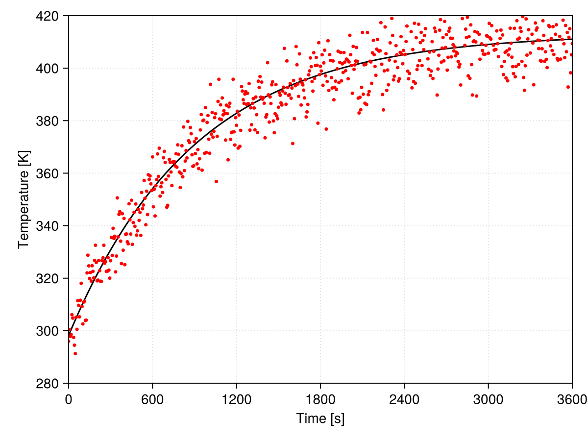
- Read
media/newton_cooling.datas a data frame - Clean data as required and establish a proper visualization
- Propose a model to fit the data and identify a package to find its parameters
Your tools:
- DataFrames
- Makie
- What else do you need?
Your goal:
30.11 Going further
Julia Documentation: in this page you find the whole documentation of Julia.
Generally after taking this short course you should be able to navigate and understand a good part of the Manual.
It is also interesting to check-out Base to explore what is built-in to Julia and avoid reinventing the wheel!
Notice that not everything built-in to Julia is available under
Baseand some functionalities are available in the Standard Library which consists of built-in packages that are shipped with Julia.
Julia Academy: you can find a few courses conceived by important Julia community members in this page. The Introduction to Julia is a longer version of what you learned here.
Python: Julia does not replace Python (yet) because it is much younger. We have seen how to call Python from Julia and the computational scientist should be well versed in both languages as of today.
Julia Packages: the ecosystem of Julia is reaching a good maturity level and you can explore it to find packages suiting your needs in this page.
Exercism Julia Track: this page proposes learning through exercises, it is good starting point to get the fundamentals of algorithmic thinking.
Julia Data Science: a very straightforward book on Data Science in Julia; you can learn more about tabular data and review some plotting with Makie here.
Introduction to Computational Thinking: this MIT course by Julia’s creator Dr. Alan Edelman gives an excellent overview of how powerful the language can be in several scientific domains.
SciML Book: this course enters more avanced topics and might be interesting as a final learning resource for those into applied mathematics and numerical simulation.
JuliaHub: this company proposes a cloud platform (non-free) for performing computations with Julia. In its page you find a few useful and good quality learning materials.
30.12 A few Julia organizations
SciML: don’t be tricked by its name, its field of application goes way beyond what we understand by Machine Learning. SciML is probably the best curated set of open source scientific tools out there. Take a look at the list of available packages here. This last link is probably the best place to search for a generic package for Scientific Computing.
JuMP: it is a modeling language for optimization problems inside Julia. It is known to work well with several SciML packages and allows to state problems in a readable way. Its documentation has its own Getting started with Julia that you may use to review this module.
JuliaData: all about tabular data and related manipulations. The parents of DataFrames.jl.
Julia Math: several math-related packages. Most basic users coming from spreadsheet hell might be interested in Polynomials.jl from this family.
JuliaMolsim: molecular simulation in Julia, from DFT to Molecular dynamics.
JuliaGeometry: computational geometry (meshes, ray tracing) packages.
30.13 Getting help in the wild
Julialang Discourse: instead of Stackoverflow, most Julia discussion threads are hosted in this page.
Zulipchat Julialang: some discussion (specially regarding development) is hold at Zulipchat.