31  Porosity quantification

In this notebook we implement a simple segmentation routine for porosity quantification.

Workflow is mostly based on scikit-image package.

You should run it sequentially and check quality of outputs at each step.

31.1 Required tools

from pathlib import Path
from skimage.io import imread
from skimage.draw import ellipse
from skimage.exposure import rescale_intensity
from skimage.filters import gaussian
from skimage.filters import threshold_otsu
from skimage.measure import find_contours
from skimage.measure import label
from skimage.measure import regionprops
from skimage.measure import regionprops_table
from skimage.transform import rotate
import warnings
import numpy as np
import matplotlib.pyplot as plt
import pandas as pd

media = Path(".").resolve().parent / "media" / "samples-porosity"
media.exists()

True

def display_img(img, cmap="gray", no_ticks=True, **kw):
    """ Display an image in a standard way with no borders. """
    fig, ax = plt.subplots()
    ax.imshow(img, cmap=cmap, **kw)

    if no_ticks:
        ax.axis("off")
        plt.subplots_adjust(left=0, right=1, top=1, bottom=0)

31.2 Load and inspect initial image

Consider providing the relative or full path to target image.

# fname = media / "500004.JPG"
# fname = media / "700005.JPG"

fname = media / "800009.JPG"
fname.exists()

True

Image is loaded in gray-scale, i.e. as a 2-D array, for later thresholding.

img0 = imread(fname, as_gray=True)

display_img(img0)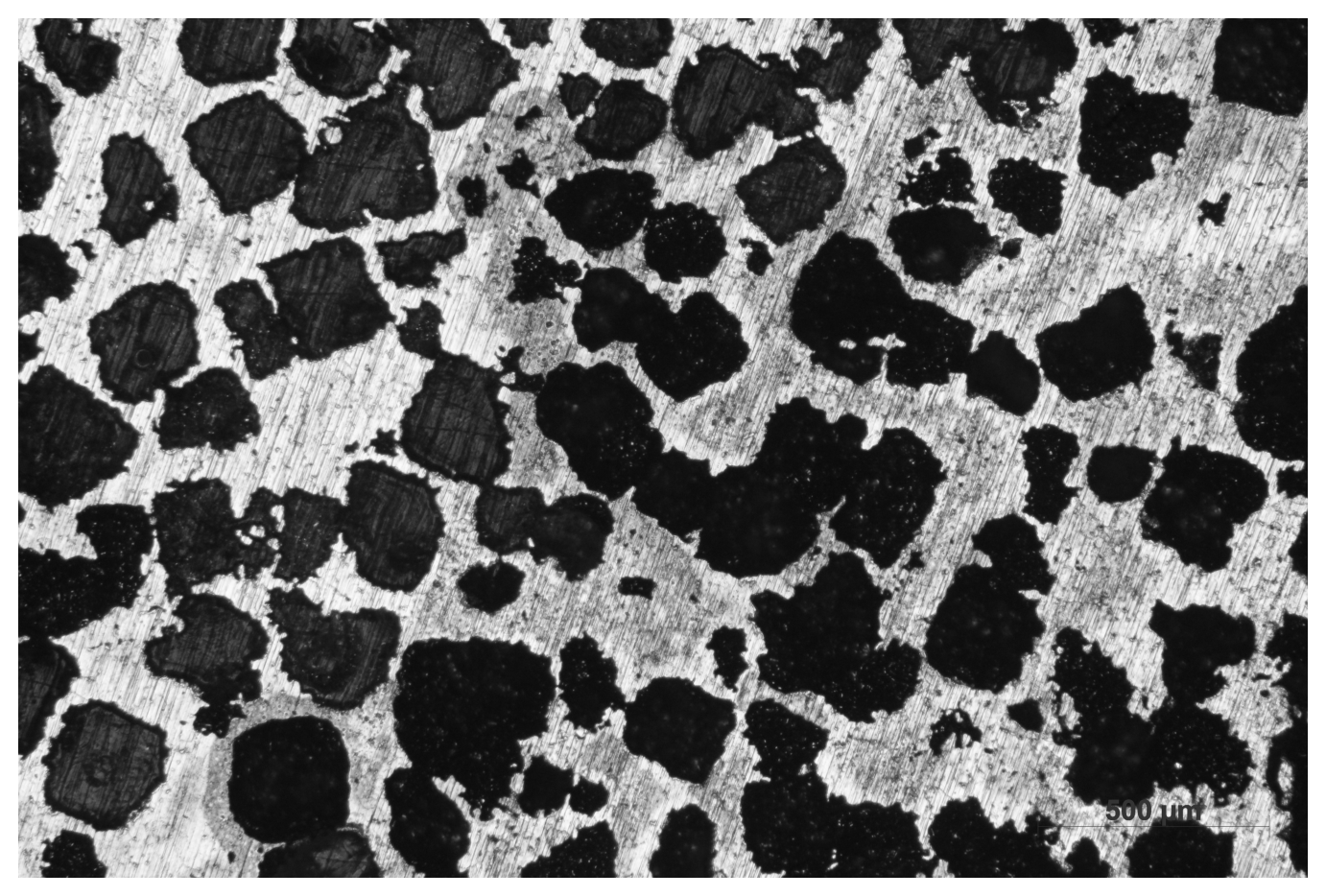

31.3 Blurring

Because of grinding and etching defects, it is important to apply an initial blur to the image.

You can control this by changing the value of sigma, the variance of the filter.

NOTE: the sigma value you choose here will impact the value of threshold img_lo you will use later. If Otsu automated thresholding works properly, you do not need to tweak this parameter and the associated img_lo. This is provided for cases where Otsu fails to automatically get pore boundaries.

img1 = gaussian(img0, sigma=15)

display_img(img1)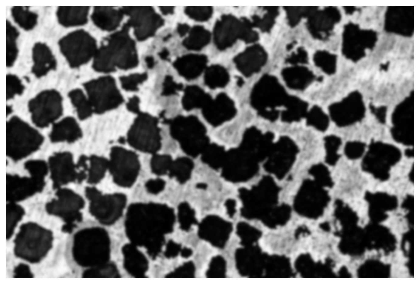

31.4 Rescaling

Rescaling with standardize the range of image for later binary selection.

There is no need to tweak the next cell.

img2 = rescale_intensity(img1, out_range=(-1, 1))

display_img(img2)

31.5 Manual thresholding

Using a cut-off lower threshold we can capture the pores.

You need to manually edit parameter img_lo, which should be close to -1 because image intensity has been scaled to \(I\in[-1,1]\).

img_lo = -0.4

img3 = np.ones_like(img2)
img3[img2 < img_lo] = 0

display_img(img3)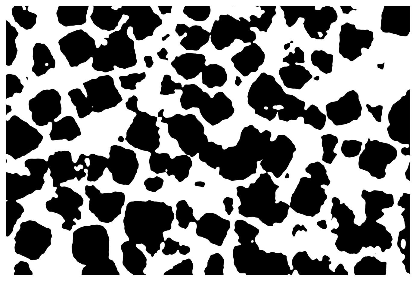

31.6 Automatic thresholding

The following is based on this example provided by scikit-image.

img4 = img1 > threshold_otsu(img1)

display_img(img4)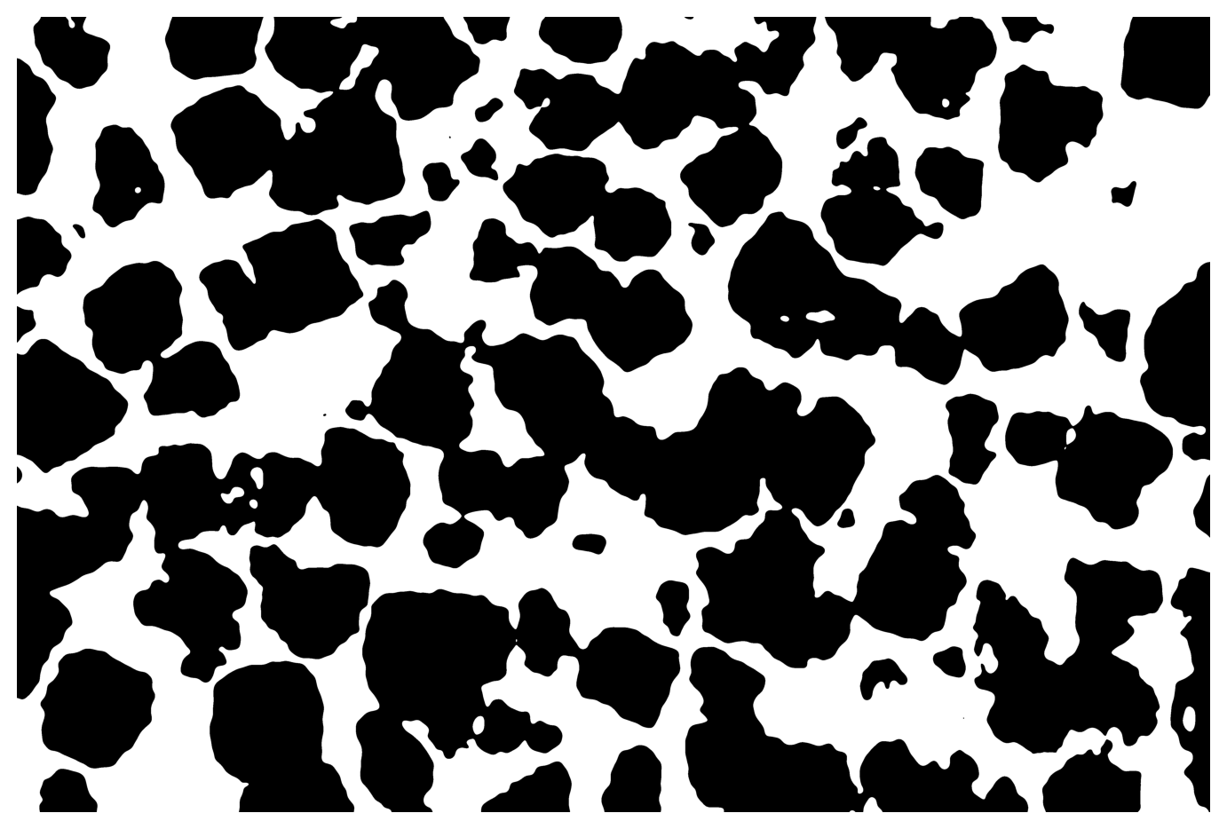

31.7 Validation and results

We find the countours of pores for display with the original image.

It is recommended you check the aspect to confirm the quality of results.

porosity_manu = 100 * (1 - img3.sum() / img0.size)
porosity_auto = 100 * (1 - img4.sum() / img0.size)

cmanu = find_contours(img3, 0.99)
cauto = find_contours(img4, 0.99)

fig, ax = plt.subplots(1, 2, figsize=(12, 6))

ax[0].set_title(f"Manual porosity of {porosity_manu:.1f}%")
ax[1].set_title(f"Automated porosity of {porosity_auto:.1f}%")

ax[0].imshow(img0, cmap="gray")
ax[1].imshow(img0, cmap="gray")

for c in cmanu:
    ax[0].plot(c[:, 1], c[:, 0], color="r", linewidth=0.5)

for c in cauto:
    ax[1].plot(c[:, 1], c[:, 0], color="r", linewidth=0.5)

ax[0].axis("off")
ax[1].axis("off")

fig.tight_layout()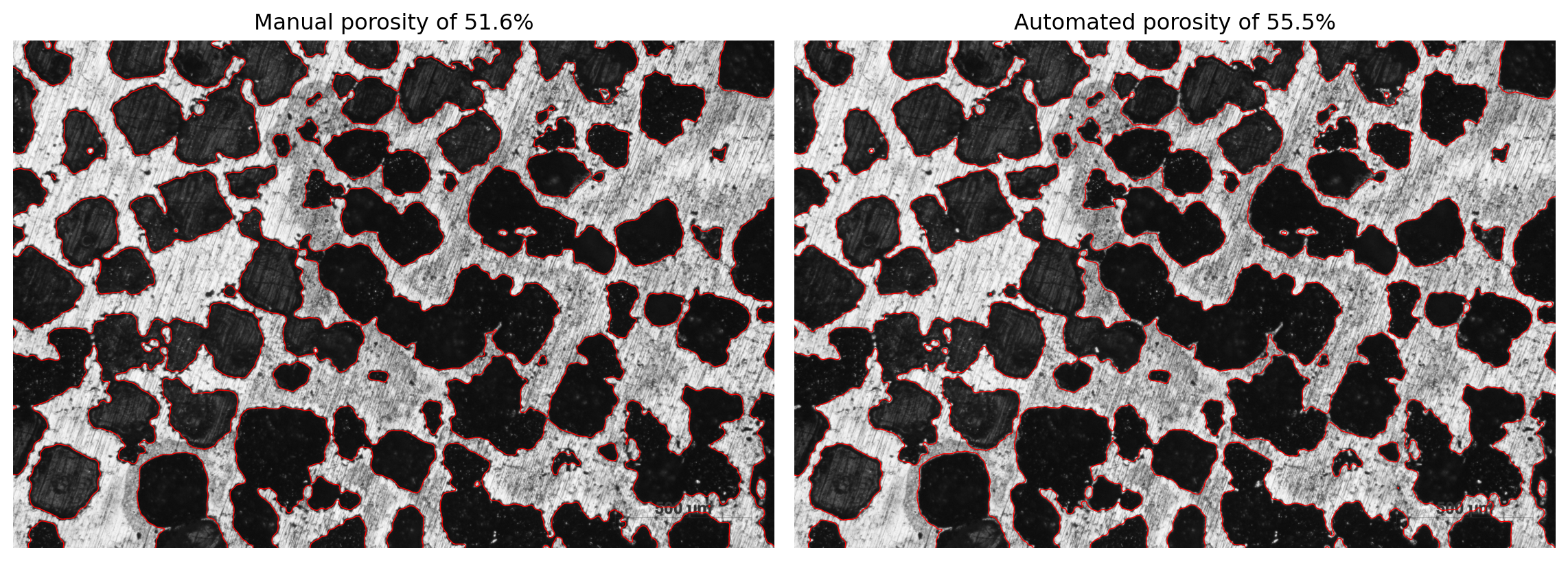

31.8 Workflow wrap-up

def porosity_workflow(fname, sigma=15):
    """ Mostly automated quantification (play with sigma). """
    img0 = imread(fname, as_gray=True)
    img1 = gaussian(img0, sigma=sigma)
    img2 = rescale_intensity(img1, out_range=(-1, 1))
    img4 = img1 > threshold_otsu(img1)

    porosity = 100 * (1 - img4.sum() / img0.size)
    contours = find_contours(img4, 0.99)

    plt.close("all")
    fig, ax = plt.subplots(1, 1, figsize=(6, 5))
    ax.set_title(f"Automated porosity of {porosity:.1f}%")
    ax.imshow(img0, cmap="gray")

    for c in contours:
        ax.plot(c[:, 1], c[:, 0], color="r", linewidth=1)

    ax.axis("off")
    fig.tight_layout()

porosity_workflow(fname)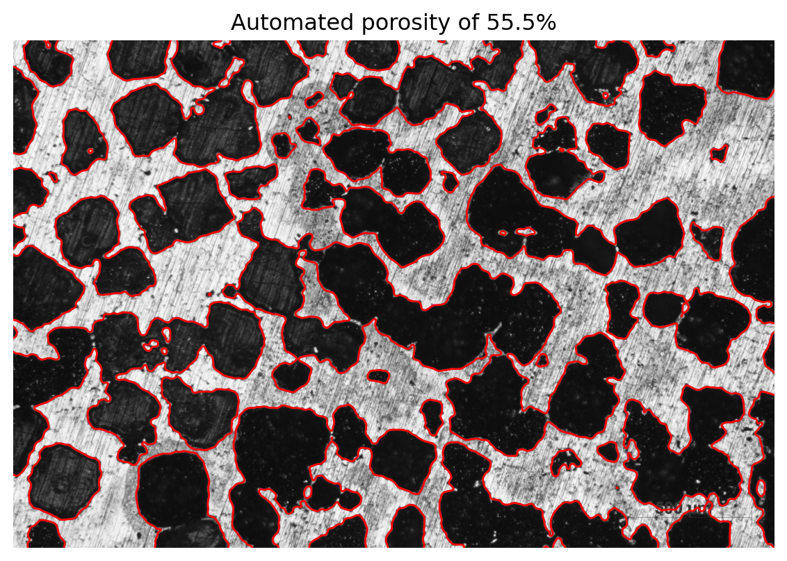

31.9 Region properties bonus

def plot_region(ax, props, cutoff):
    """ Display a region with borders and equivalent ellipse. """
    if props.area < cutoff:
        return

    y0, x0 = props.centroid
    theta = props.orientation

    x1 = x0 + np.cos(theta) * props.axis_minor_length / 2
    y1 = y0 - np.sin(theta) * props.axis_minor_length / 2
    x2 = x0 - np.sin(theta) * props.axis_major_length / 2
    y2 = y0 - np.cos(theta) * props.axis_major_length / 2

    # TODO test if not at border

    ax.plot((x0, x1), (y0, y1), "-r", linewidth=1)
    ax.plot((x0, x2), (y0, y2), "-r", linewidth=1)
    ax.plot(x0, y0, ".g", markersize=15)

    minr, minc, maxr, maxc = props.bbox
    bx = (minc, maxc, maxc, minc, minc)
    by = (minr, minr, maxr, maxr, minr)
    ax.plot(bx, by, "-b", linewidth=1)

def plot_all_regions(img, contours, regions, cutoff):
    """ Plot all detected regions in an image. """
    plt.close("all")
    fig, ax = plt.subplots(1, 1, figsize=(6, 5))
    # ax.set_title(f"Automated porosity of {porosity:.1f}%")
    ax.imshow(img, cmap="gray")

    for c in contours:
        ax.plot(c[:, 1], c[:, 0], color="y", linewidth=1)

    for props in regions:
        plot_region(ax, props, cutoff)

    ax.axis("off")
    plt.subplots_adjust(left=0, right=1, top=1, bottom=0)
    # fig.tight_layout()

    return fig, ax

def regions_workflow(fname, sigma=10, cutoff=20):
    """ Mostly automated quantification (play with sigma). """
    img0 = imread(fname, as_gray=True)
    img1 = gaussian(img0, sigma=sigma)
    img2 = rescale_intensity(img1, out_range=(-1, 1))
    img4 = img1 > threshold_otsu(img1)

    label_img = label(1 - img4)
    regions = regionprops(label_img)

    porosity = 100 * (1 - img4.sum() / img0.size)
    contours = find_contours(img4, 0.99)

    fig, ax = plot_all_regions(img0, contours, regions, cutoff)

    table = regionprops_table(label_img, properties=(
        "area",
        'axis_major_length',
        'axis_minor_length',
        'centroid',
        "eccentricity",
        "equivalent_diameter_area",
        "feret_diameter_max",
        'orientation',
        "perimeter",
        "perimeter_crofton"
    ))
    return pd.DataFrame(table)

table = regions_workflow(fname)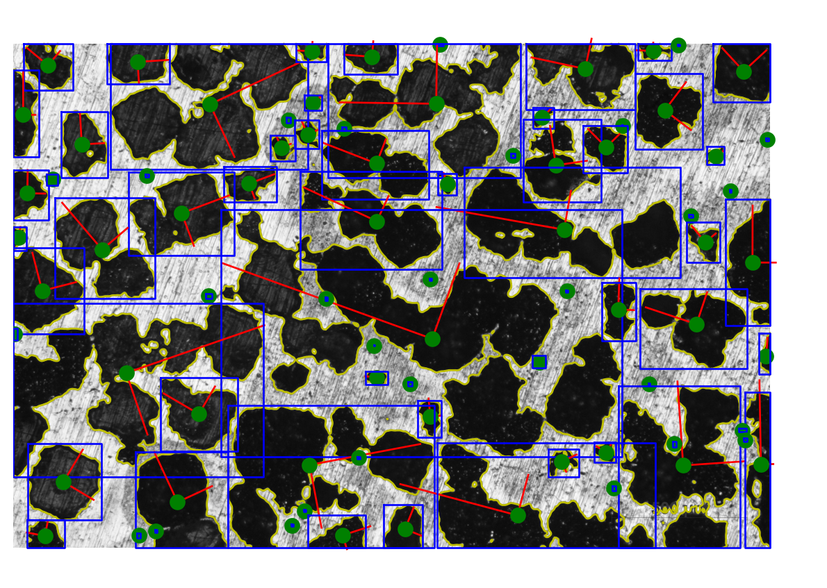

table.head().T

	0	1	2	3	4
area	73161.000000	97748.000000	665846.000000	18612.000000	60719.000000
axis_major_length	376.235279	439.661618	1353.375215	200.600567	376.278958
axis_minor_length	256.600252	293.277190	796.578811	128.380797	213.213921
centroid-0	148.098618	123.927640	414.686540	50.954760	88.785537
centroid-1	236.947486	850.714746	1345.892332	2045.305985	2456.921507
eccentricity	0.731333	0.745011	0.808434	0.768390	0.823967
equivalent_diameter_area	305.207271	352.784097	920.750486	153.940035	278.046456
feret_diameter_max	378.498349	453.007726	1383.046275	216.094887	368.401954
orientation	0.875968	-1.507255	-1.134392	1.518901	1.495124
perimeter	1270.856998	1292.482323	6860.861720	611.297511	1013.955411
perimeter_crofton	1207.529502	1228.031596	6504.701132	582.424248	963.971525

For post-processing, now you can think about anything, such as creating bins for classification:

table["classes"] = pd.cut(table["area"], bins=4)
table.groupby("classes", observed=True).agg(("count", "mean", "std")).T.head(6)

	classes	(-1694.008, 424255.0]	(424255.0, 848507.0]	(1272759.0, 1697011.0]
area	count	74.000000	7.000000	1.000000e+00
	mean	54913.635135	604669.142857	1.697011e+06
	std	80866.246036	137960.255980	NaN
axis_major_length	count	74.000000	7.000000	1.000000e+00
	mean	259.567942	1544.173949	3.048717e+03
	std	281.790113	293.199681	NaN