%load_ext autoreload
%autoreload 227 Inviscid Bump in a Channel
This notebook provides a Python approach to setup and run the standard tutorial case Inviscid Bump and reading that case before getting here is highly recommended, since we will not be discussing all the points.
The main goal is provide a full Python interface to the problem from case construction to post-processing. This is done through our package majordome and pyvista, an excellent tool for VTK data rendering. Alternative approaches of VTK data rendering are discussed here.
Next we configure pv to display static images in notebook. We also start the display.
from majordome.su2.mesh import *
from majordome.su2.enums import *
from majordome.su2.groups import *
import pyvista as pv

pv.set_jupyter_backend("static")
C:\Users\walte\GitHub\majordome\notes\.venv\Lib\site-packages\rsciio\utils\rgb_tools.py:46: VisibleDeprecationWarning: The module `rsciio.utils.rgb_tools` has been renamed to `rsciio.utils.rgb` and it will be removed in version 1.0.
warnings.warn(
C:\Users\walte\GitHub\majordome\notes\.venv\Lib\site-packages\rsciio\utils\tools.py:93: VisibleDeprecationWarning: ensure_directory has been moved to `rsciio.utils.path` and will be removed from `rsciio.utils.tools` in version 1.0.
warnings.warn(message, VisibleDeprecationWarning)
C:\Users\walte\GitHub\majordome\notes\.venv\Lib\site-packages\rsciio\utils\tools.py:93: VisibleDeprecationWarning: append2pathname has been moved to `rsciio.utils.path` and will be removed from `rsciio.utils.tools` in version 1.0.
warnings.warn(message, VisibleDeprecationWarning)
C:\Users\walte\GitHub\majordome\notes\.venv\Lib\site-packages\rsciio\utils\tools.py:93: VisibleDeprecationWarning: incremental_filename has been moved to `rsciio.utils.path` and will be removed from `rsciio.utils.tools` in version 1.0.
warnings.warn(message, VisibleDeprecationWarning)
C:\Users\walte\GitHub\majordome\notes\.venv\Lib\site-packages\tqdm\auto.py:21: TqdmWarning: IProgress not found. Please update jupyter and ipywidgets. See https://ipywidgets.readthedocs.io/en/stable/user_install.html
from .autonotebook import tqdm as notebook_tqdm
C:\Users\walte\GitHub\majordome\notes\.venv\Lib\site-packages\rsciio\utils\tools.py:93: VisibleDeprecationWarning: ensure_directory has been moved to `rsciio.utils.path` and will be removed from `rsciio.utils.tools` in version 1.0.
warnings.warn(message, VisibleDeprecationWarning)
C:\Users\walte\GitHub\majordome\notes\.venv\Lib\site-packages\rsciio\utils\tools.py:93: VisibleDeprecationWarning: overwrite has been moved to `rsciio.utils.path` and will be removed from `rsciio.utils.tools` in version 1.0.
warnings.warn(message, VisibleDeprecationWarning)27.1 Domain inspection
As of any CFD problem, visualization is of utmost importance. Using pyvista we provide below the rendering of problem mesh.
From the outline property we can get a good guess of camera placement to see the mesh later.
mesh_reader = SU2MeshLoader("mesh.su2")
mesh = mesh_reader.to_pyvista()
mesh.outline()
Warning: meshio does not support tags of string type. Surface tag inlet will be replaced by 1
Warning: meshio does not support tags of string type.
    Surface tag  lower_wall will be replaced by 2
Warning: meshio does not support tags of string type.
    Surface tag  outlet will be replaced by 3
Warning: meshio does not support tags of string type.
    Surface tag  upper_wall will be replaced by 4
| PolyData | Information |
|---|---|
| N Cells | 12 |
| N Points | 8 |
| N Strips | 0 |
| X Bounds | 0.000e+00, 3.000e+00 |
| Y Bounds | 0.000e+00, 1.000e+00 |
| Z Bounds | 0.000e+00, 0.000e+00 |
| N Arrays | 0 |
class ExtendedPlotter:
    """ A wrapper around pyvista.Plotter to set some default options. """
    def __init__(self, *args, **kwargs):
        self.plotter = pv.Plotter(*args, **kwargs)

    def add_mesh(self, *args, **kwargs):
        self.plotter.add_mesh(*args, **kwargs)

    def show(self, *args, **kwargs):
        bg = kwargs.pop("background", "#CCCCCC")
        ps = kwargs.pop("parallel_scale", 1.2)

        self.plotter.renderer.set_background(bg)
        self.plotter.renderer.reset_camera()
        self.plotter.camera.zoom("tight")
        self.plotter.camera.parallel_scale *= ps

        self.plotter.show(*args, **kwargs)

    @property
    def renderer(self):
        return self.plotter.renderer

    @property
    def camera(self):
        return self.plotter.camera
# XXX: casting required to avoid linting warnings:
p = ExtendedPlotter()
p.add_mesh(mesh.cast_to_unstructured_grid(), show_edges=True, color="w")
p.show()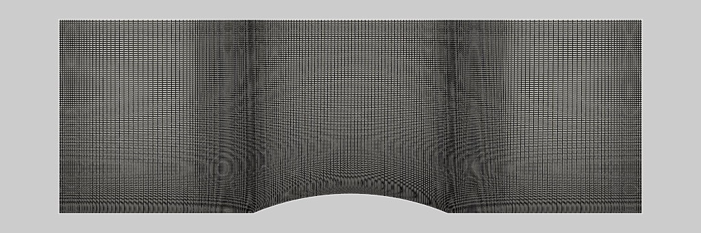
With boundaries in hand we can use a more complex feature of pyvista to make a composite plot depicting each of these selected tags. A grid is also added to the image to provide the size of the system, which will later also be need to analyse the data.
mesh_grid      = mesh#.cast_to_unstructured_grid()
tag_inlet      = mesh_reader.get_tag("inlet")
tag_lower_wall = mesh_reader.get_tag("lower_wall")
tag_outlet     = mesh_reader.get_tag("outlet")
tag_upper_wall = mesh_reader.get_tag("upper_wall")
p = ExtendedPlotter()
p.add_mesh(mesh_grid, color="w", show_edges=True, opacity=0.3)
p.add_mesh(tag_inlet, color="r", show_edges=True, line_width=5)
p.add_mesh(tag_lower_wall, color="g", show_edges=True, line_width=5)
p.add_mesh(tag_outlet, color="b", show_edges=True, line_width=5)
p.add_mesh(tag_upper_wall, color="g", show_edges=True, line_width=5)
p.renderer.show_grid(xtitle="X", ytitle="Y", font_size=20,
color="k", bold=True,)
p.show(parallel_scale=1.4)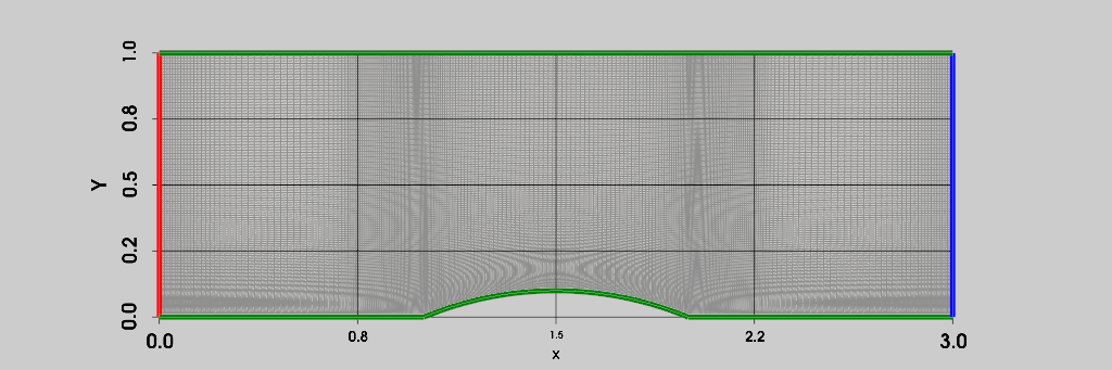
27.2 Prepare case configuration
In this section we show how to use majordome to transform the original case into a Python script. This has the advantage to allow parametric generation of cases and other computations to be performed directly in case construction. Different sections of SU2 configuration files are simply filled-in through Python classes as follows. Dumping of .cfg file is automatically manager by SU2Configuration.
conf = SU2Configuration(
    problem = ProblemDefinition(
        solver = SolverType.EULER,
    )
)

conf.compressible_freestream = CompressibleFreeStreamDefinition(
    mach             = 0.5,
    angle_of_attack  = 0.0,
    sideslip_angle   = 0.0,
    pressure         = 101325.0,
    temperature      = 288.0
)

conf.reference_values = ReferenceValues(
    ref_origin_moment_x = 0.25,
    ref_origin_moment_y = 0.00,
    ref_origin_moment_z = 0.00,
    ref_length          = 1.0,
    ref_area            = 1.0
)

conf.boundary_conditions = BoundaryConditions(
    marker_euler  = [
        BCTypeWallEuler("upper_wall"),
        BCTypeWallEuler("lower_wall"),
    ],
    marker_inlet  = ["inlet", 288.6, 102010.0, 1.0, 0.0, 0.0],
    marker_outlet = ["outlet", 101300.0],
    inlet_type    = InletType.TOTAL_CONDITIONS,
)

conf.surfaces_identification = SurfacesIdentification(
    marker_plotting   = ["lower_wall"],
    marker_monitoring = ["upper_wall", "lower_wall"],
)

conf.common_numerical_parameters = CommonParametersNumerical(
    num_method_grad = NumMethodGrad.GREEN_GAUSS,
    cfl_number      = 50.0,
    cfl_adapt       = YesNoEnum.YES,
    cfl_adapt_param = ParametersCFL(
        factor_down            = 0.1,
        factor_up              = 2.0,
        min_value              = 50.0,
        max_value              = 1.0e+10
    ),
    rk_alpha_coeff = (0.66667, 0.66667, 1.000000),
)

conf.linear_solver_parameters = LinearSolverParameters(
    linear_solver      = LinearSolver.FGMRES,
    linear_solver_prec = Preconditioner.ILU,
    error              = 1.0e-10,
    n_iter             = 20
)

conf.multigrid_parameters = MultigridParameters(
    mg_level             = 3,
    mg_cycle             = MgCycle.W_CYCLE,
    mg_pre_smooth        = [1, 2, 3, 3],
    mg_post_smooth       = [0, 0, 0, 0],
    mg_correction_smooth = [0, 0, 0, 0],
    mg_damp_restriction  = 1.0,
    mg_damp_prolongation = 1.0
)

conf.flow_numerical_method = FlowNumericalMethod(
    conv_num_method_flow = ConvectiveScheme.JST,
    time_discre_flow     = TimeDiscretization.EULER_IMPLICIT,
)

conf.slope_limiter = SlopeLimiter(
    jst_sensor_coeff = (0.5, 0.02)
)

conf.solver_control = SolverControl(
    iter                 = 999999,
    conv_field           = "RMS_DENSITY",
    conv_residual_minval = -10,
    conv_startiter       = 10,
    conv_cauchy_elems    = 100,
    conv_cauchy_eps      = 1.0e-10,
)

conf.screen_history_info = ScreenHistoryInfo(
    screen_output = [
        "INNER_ITER",
        "WALL_TIME",
        "RMS_DENSITY",
        "RMS_ENERGY",
        "LIFT",
        "DRAG"
    ],
)

conf.io_file_info = IOFileInfo(
    mesh_filename         = "mesh.su2",
    mesh_format           = MeshFormat.SU2,
    mesh_out_filename     = "mesh_out.su2",
    solution_filename     = "solution_flow",
    solution_adj_filename = "solution_adj",
    tabular_format        = TabularFormat.CSV,
    conv_filename         = "history.dat",
    restart_filename      = "restart_flow",
    restart_adj_filename  = "restart_adj",
    volume_filename       = "flow",
    volume_adj_filename   = "adjoint",
    grad_objfunc_filename = "of_grad.dat",
    surface_filename      = "surface_flow",
    surface_adj_filename  = "surface_adjoint",
)

conf.to_file("model.cfg", force=True)
Before going to the next section, let’s make a dry run for verification of configuration file:
!SU2_CFD -d model.cfg
-------------------------------------------------------------------------
| ___ _ _ ___ |
| / __| | | |_ ) Release 8.3.0 "Harrier" |
| \__ \ |_| |/ / |
| |___/\___//___| Suite (Computational Fluid Dynamics Code) |
| |
-------------------------------------------------------------------------
| SU2 Project Website: https://su2code.github.io |
| |
| The SU2 Project is maintained by the SU2 Foundation |
| (http://su2foundation.org) |
-------------------------------------------------------------------------
| Copyright 2012-2025, SU2 Contributors |
| |
| SU2 is free software; you can redistribute it and/or |
| modify it under the terms of the GNU Lesser General Public |
| License as published by the Free Software Foundation; either |
| version 2.1 of the License, or (at your option) any later version. |
| |
| SU2 is distributed in the hope that it will be useful, |
| but WITHOUT ANY WARRANTY; without even the implied warranty of |
| MERCHANTABILITY or FITNESS FOR A PARTICULAR PURPOSE. See the GNU |
| Lesser General Public License for more details. |
| |
| You should have received a copy of the GNU Lesser General Public |
| License along with SU2. If not, see <http://www.gnu.org/licenses/>. |
-------------------------------------------------------------------------
Parsing config file for zone 0
----------------- Physical Case Definition ( Zone 0 ) -------------------
Compressible Euler equations.
Mach number: 0.5.
Angle of attack (AoA): 0 deg, and angle of sideslip (AoS): 0 deg.
No restart solution, use the values at infinity (freestream).
Dimensional simulation.
The reference area is 1 m^2.
The semi-span will be computed using the max y(3D) value.
The reference length is 1 m.
Surface(s) where the force coefficients are evaluated and
their reference origin for moment computation:
- upper_wall (0.25, 0, 0).
- lower_wall (0.25, 0, 0) m.
Surface(s) plotted in the output file: lower_wall.
Input mesh file name: mesh.su2
--------------- Space Numerical Integration ( Zone 0 ) ------------------
Jameson-Schmidt-Turkel scheme (2nd order in space) for the flow inviscid terms.
JST viscous coefficients (2nd & 4th): 0.5, 0.02.
The method includes a grid stretching correction (p = 0.3).
Gradient for upwind reconstruction: Green-Gauss.
Gradient for viscous and source terms: Green-Gauss.
--------------- Time Numerical Integration ( Zone 0 ) ------------------
Local time stepping (steady state simulation).
Euler implicit method for the flow equations.
FGMRES is used for solving the linear system.
Using a ILU(0) preconditioning.
Convergence criteria of the linear solver: 1e-10.
Max number of linear iterations: 20.
W Multigrid Cycle, with 3 multigrid levels.
Damping factor for the residual restriction: 1.
Damping factor for the correction prolongation: 1.
CFL adaptation. Factor down: 0.1, factor up: 2,
lower limit: 50, upper limit: 1e+10,
acceptable linear residual: 0.001'
starting iteration: 0.
+-------------------------------------------+
| MG Level| Presmooth|PostSmooth|CorrectSmo|
+-------------------------------------------+
| 0| 1| 0| 0|
| 1| 2| 0| 0|
| 2| 3| 0| 0|
| 3| 3| 0| 0|
+-------------------------------------------+
Courant-Friedrichs-Lewy number: 50
------------------ Convergence Criteria ( Zone 0 ) ---------------------
Maximum number of solver subiterations: 999999.
Begin convergence monitoring at iteration 10.
Residual minimum value: 1e-10.
Cauchy series min. value: 1e-10.
Number of Cauchy elements: 100.
Begin windowed time average at iteration 0.
-------------------- Output Information ( Zone 0 ) ----------------------
File writing frequency:
+------------------------------------+
| File| Frequency|
+------------------------------------+
| RESTART| 250|
| PARAVIEW| 250|
| SURFACE_PARAVIEW| 250|
+------------------------------------+
Writing the convergence history file every 1 inner iterations.
Writing the screen convergence history every 1 inner iterations.
The tabular file format is CSV (.csv).
Convergence history file name: history.dat.
Forces breakdown file name: forces_breakdown.dat.
Surface file name: surface_flow.
Volume file name: flow.
Restart file name: restart_flow.
------------- Config File Boundary Information ( Zone 0 ) ---------------
+-----------------------------------------------------------------------+
| Marker Type| Marker Name|
+-----------------------------------------------------------------------+
| Euler wall| upper_wall|
| | lower_wall|
+-----------------------------------------------------------------------+
| Inlet boundary| inlet|
+-----------------------------------------------------------------------+
| Outlet boundary| outlet|
+-----------------------------------------------------------------------+
-------------------- Output Preprocessing ( Zone 0 ) --------------------
WARNING: SURFACE_PRESSURE_DROP can only be computed for at least 2 surfaces (outlet, inlet, ...)
Screen output fields: INNER_ITER, WALL_TIME, RMS_DENSITY, RMS_ENERGY, LIFT, DRAG
History output group(s): ITER, RMS_RES
Convergence field(s): RMS_DENSITY
Warning: No (valid) fields chosen for time convergence monitoring. Time convergence monitoring inactive.
Volume output fields: COORDINATES, SOLUTION, PRIMITIVE
-------------------------- Using Dummy Geometry -------------------------
Computing wall distances.
-------------------- Solver Preprocessing ( Zone 0 ) --------------------
Inviscid flow: Computing density based on free-stream
temperature and pressure using the ideal gas law.
Force coefficients computed using free-stream values.
-- Models:
+------------------------------------------------------------------------------+
| Viscosity Model| Conductivity Model| Fluid Model|
+------------------------------------------------------------------------------+
| -| -| STANDARD_AIR|
+------------------------------------------------------------------------------+
-- Fluid properties:
+------------------------------------------------------------------------------+
| Name| Dim. value| Ref. value| Unit|Non-dim. value|
+------------------------------------------------------------------------------+
| Gas Constant| 287.058| 1| N.m/kg.K| 287.058|
| Spec. Heat Ratio| -| -| -| 1.4|
+------------------------------------------------------------------------------+
-- Initial and free-stream conditions:
+------------------------------------------------------------------------------+
| Name| Dim. value| Ref. value| Unit|Non-dim. value|
+------------------------------------------------------------------------------+
| Static Pressure| 101325| 1| Pa| 101325|
| Density| 1.22562| 1| kg/m^3| 1.22562|
| Temperature| 288| 1| K| 288|
| Total Energy| 221149| 1| m^2/s^2| 221149|
| Velocity-X| 170.104| 1| m/s| 170.104|
| Velocity-Y| 0| 1| m/s| 0|
| Velocity Magnitude| 170.104| 1| m/s| 170.104|
+------------------------------------------------------------------------------+
| Mach Number| -| -| -| 0.5|
+------------------------------------------------------------------------------+
Initialize Jacobian structure (Euler). MG level: 0.
Initialize Jacobian structure (Euler). MG level: 1.
Initialize Jacobian structure (Euler). MG level: 2.
Initialize Jacobian structure (Euler). MG level: 3.
------------------- Numerics Preprocessing ( Zone 0 ) -------------------
----------------- Integration Preprocessing ( Zone 0 ) ------------------
------------------- Iteration Preprocessing ( Zone 0 ) ------------------
Euler/Navier-Stokes/RANS fluid iteration.
------------------------------ Begin Solver -----------------------------
--------------------------------------------
No solver started. DRY_RUN option enabled.
--------------------------------------------
Available volume output fields for the current configuration in Zone 0 (Comp. Fluid):
Note: COORDINATES are always included, and so is SOLUTION unless you add the keyword COMPACT to the list of fields.
+----------------------------------------------------------------------------------+
|Name |Group Name |Description |
+----------------------------------------------------------------------------------+
|COORD-X |COORDINATES |x-component of the coordinate vector |
|COORD-Y |COORDINATES |y-component of the coordinate vector |
|DENSITY |SOLUTION |Density |
|MOMENTUM-X |SOLUTION |x-component of the momentum vector |
|MOMENTUM-Y |SOLUTION |y-component of the momentum vector |
|ENERGY |SOLUTION |Energy |
|PRESSURE |PRIMITIVE |Pressure |
|TEMPERATURE |PRIMITIVE |Temperature |
|MACH |PRIMITIVE |Mach number |
|PRESSURE_COEFF |PRIMITIVE |Pressure coefficient |
|VELOCITY-X |PRIMITIVE |x-component of the velocity vector |
|VELOCITY-Y |PRIMITIVE |y-component of the velocity vector |
|RES_DENSITY |RESIDUAL |Residual of the density |
|RES_MOMENTUM-X |RESIDUAL |Residual of the x-momentum component |
|RES_MOMENTUM-Y |RESIDUAL |Residual of the y-momentum component |
|RES_ENERGY |RESIDUAL |Residual of the energy |
|DELTA_TIME |TIMESTEP |Value of the local timestep for the flow variables|
|CFL |TIMESTEP |Value of the local CFL for the flow variables |
|ROE_DISSIPATION|ROE_DISSIPATION|Value of the Roe dissipation |
|ORTHOGONALITY |MESH_QUALITY |Orthogonality Angle (deg.) |
|ASPECT_RATIO |MESH_QUALITY |CV Face Area Aspect Ratio |
|VOLUME_RATIO |MESH_QUALITY |CV Sub-Volume Ratio |
|RANK |MPI |Rank of the MPI-partition |
|MG_1 |MULTIGRID |Coarse mesh |
|MG_2 |MULTIGRID |Coarse mesh |
|MG_3 |MULTIGRID |Coarse mesh |
+----------------------------------------------------------------------------------+
Available screen/history output fields for the current configuration in Zone 0 (Comp. Fluid):
+---------------------------------------------------------------------------------------------------------------------------+
|Name |Group Name |Type |Description |
+---------------------------------------------------------------------------------------------------------------------------+
|TIME_ITER |ITER |D |Time iteration index |
|OUTER_ITER |ITER |D |Outer iteration index |
|INNER_ITER |ITER |D |Inner iteration index |
|CUR_TIME |TIME_DOMAIN |D |Current physical time (s) |
|TIME_STEP |TIME_DOMAIN |D |Current time step (s) |
|WALL_TIME |WALL_TIME |D |Average wall-clock time since the start of inner iterations. |
|NONPHYSICAL_POINTS |NONPHYSICAL_POINTS|D |The number of non-physical points in the solution |
|RMS_DENSITY |RMS_RES |R |Root-mean square residual of the density. |
|RMS_MOMENTUM-X |RMS_RES |R |Root-mean square residual of the momentum x-component. |
|RMS_MOMENTUM-Y |RMS_RES |R |Root-mean square residual of the momentum y-component. |
|RMS_ENERGY |RMS_RES |R |Root-mean square residual of the energy. |
|MAX_DENSITY |MAX_RES |R |Maximum square residual of the density. |
|MAX_MOMENTUM-X |MAX_RES |R |Maximum square residual of the momentum x-component. |
|MAX_MOMENTUM-Y |MAX_RES |R |Maximum square residual of the momentum y-component. |
|MAX_ENERGY |MAX_RES |R |Maximum residual of the energy. |
|BGS_DENSITY |BGS_RES |R |BGS residual of the density. |
|BGS_MOMENTUM-X |BGS_RES |R |BGS residual of the momentum x-component. |
|BGS_MOMENTUM-Y |BGS_RES |R |BGS residual of the momentum y-component. |
|BGS_ENERGY |BGS_RES |R |BGS residual of the energy. |
|LINSOL_ITER |LINSOL |D |Number of iterations of the linear solver. |
|LINSOL_RESIDUAL |LINSOL |D |Residual of the linear solver. |
|MIN_DELTA_TIME |CFL_NUMBER |D |Current minimum local time step |
|MAX_DELTA_TIME |CFL_NUMBER |D |Current maximum local time step |
|MIN_CFL |CFL_NUMBER |D |Current minimum of the local CFL numbers |
|MAX_CFL |CFL_NUMBER |D |Current maximum of the local CFL numbers |
|AVG_CFL |CFL_NUMBER |D |Current average of the local CFL numbers |
|SURFACE_MASSFLOW |FLOW_COEFF |C |Total average mass flow on all markers set in MARKER_ANALYZE |
|SURFACE_MACH |FLOW_COEFF |C |Total average mach number on all markers set in MARKER_ANALYZE |
|SURFACE_STATIC_TEMPERATURE |FLOW_COEFF |C |Total average temperature on all markers set in MARKER_ANALYZE |
|SURFACE_STATIC_PRESSURE |FLOW_COEFF |C |Total average pressure on all markers set in MARKER_ANALYZE |
|AVG_DENSITY |FLOW_COEFF |C |Total average density on all markers set in MARKER_ANALYZE |
|AVG_ENTHALPY |FLOW_COEFF |C |Total average enthalpy on all markers set in MARKER_ANALYZE |
|AVG_NORMALVEL |FLOW_COEFF |C |Total average normal velocity on all markers set in MARKER_ANALYZE |
|SURFACE_UNIFORMITY |FLOW_COEFF |C |Total flow uniformity on all markers set in MARKER_ANALYZE |
|SURFACE_SECONDARY |FLOW_COEFF |C |Total secondary strength on all markers set in MARKER_ANALYZE |
|SURFACE_MOM_DISTORTION |FLOW_COEFF |C |Total momentum distortion on all markers set in MARKER_ANALYZE |
|SURFACE_SECOND_OVER_UNIFORM|FLOW_COEFF |C |Total secondary over uniformity on all markers set in MARKER_ANALYZE |
|SURFACE_TOTAL_TEMPERATURE |FLOW_COEFF |C |Total average total temperature all markers set in MARKER_ANALYZE |
|SURFACE_TOTAL_PRESSURE |FLOW_COEFF |C |Total average total pressure on all markers set in MARKER_ANALYZE |
|REFERENCE_FORCE |AERO_COEFF |C |Reference force used to compute aerodynamic coefficients |
|DRAG |AERO_COEFF |C |Total drag coefficient on all surfaces set with MARKER_MONITORING |
|LIFT |AERO_COEFF |C |Total lift coefficient on all surfaces set with MARKER_MONITORING |
|SIDEFORCE |AERO_COEFF |C |Total sideforce coefficient on all surfaces set with MARKER_MONITORING|
|MOMENT_X |AERO_COEFF |C |Total momentum x-component on all surfaces set with MARKER_MONITORING |
|MOMENT_Y |AERO_COEFF |C |Total momentum y-component on all surfaces set with MARKER_MONITORING |
|MOMENT_Z |AERO_COEFF |C |Total momentum z-component on all surfaces set with MARKER_MONITORING |
|FORCE_X |AERO_COEFF |C |Total force x-component on all surfaces set with MARKER_MONITORING |
|FORCE_Y |AERO_COEFF |C |Total force y-component on all surfaces set with MARKER_MONITORING |
|FORCE_Z |AERO_COEFF |C |Total force z-component on all surfaces set with MARKER_MONITORING |
|EFFICIENCY |AERO_COEFF |C |Total lift-to-drag ratio on all surfaces set with MARKER_MONITORING |
|AOA |AOA |D |Angle of attack |
|COMBO |COMBO |C |Combined obj. function value. |
|FIGURE_OF_MERIT |ROTATING_FRAME |C |Thrust over torque |
|THRUST |ROTATING_FRAME |C |Thrust coefficient |
|TORQUE |ROTATING_FRAME |C |Torque coefficient |
|INVERSE_DESIGN_PRESSURE |CP_DIFF |C |Cp difference for inverse design |
|EQUIVALENT_AREA |EQUIVALENT_AREA |C |Equivalent area |
|DRAG_ON_SURFACE |AERO_COEFF_SURF |C | |
|LIFT_ON_SURFACE |AERO_COEFF_SURF |C | |
|SIDEFORCE_ON_SURFACE |AERO_COEFF_SURF |C | |
|MOMENT-X_ON_SURFACE |AERO_COEFF_SURF |C | |
|MOMENT-Y_ON_SURFACE |AERO_COEFF_SURF |C | |
|MOMENT-Z_ON_SURFACE |AERO_COEFF_SURF |C | |
|FORCE-X_ON_SURFACE |AERO_COEFF_SURF |C | |
|FORCE-Y_ON_SURFACE |AERO_COEFF_SURF |C | |
|FORCE-Z_ON_SURFACE |AERO_COEFF_SURF |C | |
|EFFICIENCY_ON_SURFACE |AERO_COEFF_SURF |C | |
+---------------------------------------------------------------------------------------------------------------------------+
Type legend: Default (D), Residual (R), Coefficient (C)
Generated screen/history fields (only first field of every group is shown):
+---------------------------------------------------------------------------------------------------------------------------+
|Name |Group Name |Type |Description |
+---------------------------------------------------------------------------------------------------------------------------+
|REL_RMS_DENSITY |REL_RMS_RES |AR |Relative residual. |
|REL_MAX_DENSITY |REL_MAX_RES |AR |Relative residual. |
|REL_BGS_DENSITY |REL_BGS_RES |AR |Relative residual. |
|AVG_BGS_RES |AVG_BGS_RES |AR |Average residual over all solution variables. |
|AVG_MAX_RES |AVG_MAX_RES |AR |Average residual over all solution variables. |
|AVG_RMS_RES |AVG_RMS_RES |AR |Average residual over all solution variables. |
+---------------------------------------------------------------------------------------------------------------------------+
--------------------------- Finalizing Solver ---------------------------
Deleted CNumerics container.
Deleted CIntegration container.
Deleted CSolver container.
Deleted CIteration container.
Deleted CInterface container.
Deleted CGeometry container.
Deleted CFreeFormDefBox class.
Deleted CSurfaceMovement class.
Deleted CVolumetricMovement class.
Deleted CConfig container.
Deleted nInst container.
Deleted COutput class.
-------------------------------------------------------------------------
------------------------- Exit Success (SU2_CFD) ------------------------
27.3 Run simulation
# !SU2_CFD model.cfg
# Run in 4 cores:
# !mpirun -n 4 SU2_CFD model.cfg
# !mpiexec -n 4 SU2_CFD model.cfg
# Run using all available hardware threads:
# !mpirun --use-hwthread-cpus -parallel model.cfg
# Use SU2 script to run in parallel:
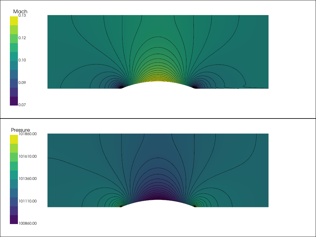
# !python3 -m parallel_computation -f model.cfg -n 2 -c COMPUTE27.4 Post-processing
grid = pv.read("flow.vtu")
# grid # uncomment to see mesh info
cpos = ((1.5, 0.4, 3.0),
(1.5, 0.4, 0.0),
(0.0, 0.0, 0.0))
vbar = {
"vertical": True,
"title_font_size": 16,
"label_font_size": 12,
"position_x": 0.03,
"position_y": 0.10,
"color": "k",
"n_colors": 10,
"width": 0.07,
"height": 0.8,
}
hbar = {
"vertical": False,
"title_font_size": 16,
"label_font_size": 12,
"position_x": 0.1,
"position_y": 0.05,
"color": "k",
"n_colors": 10,
"width": 0.8,
"height": 0.1,
}
opts = {"pbr": False, "cmap": "viridis", "scalar_bar_args": vbar}
lims1 = (100860, 101860)
opts1 = {**opts}
opts1["scalar_bar_args"]["fmt"] = "%.0f"
contour1 = grid.contour(40, scalars="Pressure", rng=lims1)
lims2 = (0.07, 0.13)
opts2 = {**opts}
opts2["scalar_bar_args"]["fmt"] = "%.2f"
contour2 = grid.contour(40, scalars="Mach", rng=lims2)
p = pv.Plotter(shape="1/1")
p.renderer.set_background(color="w")
p.subplot(0)
p.add_mesh(grid.cast_to_unstructured_grid(), **opts1, scalars="Pressure", clim=lims1)
p.add_mesh(contour1, color="k", line_width=1)
p.subplot(1)
p.add_mesh(grid.cast_to_unstructured_grid(), **opts2, scalars="Mach", clim=lims2)
p.add_mesh(contour2, color="k", line_width=1)
p.link_views()
p.show(cpos=cpos)